Firm Decisions in the Long Run I
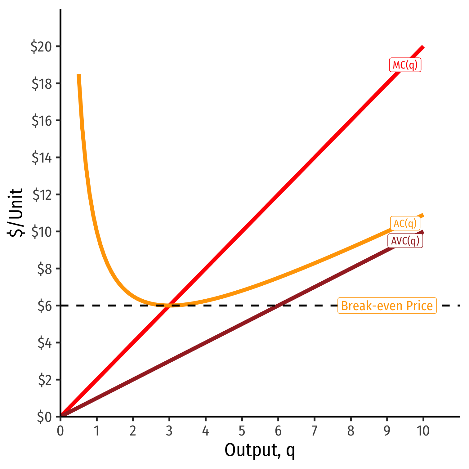
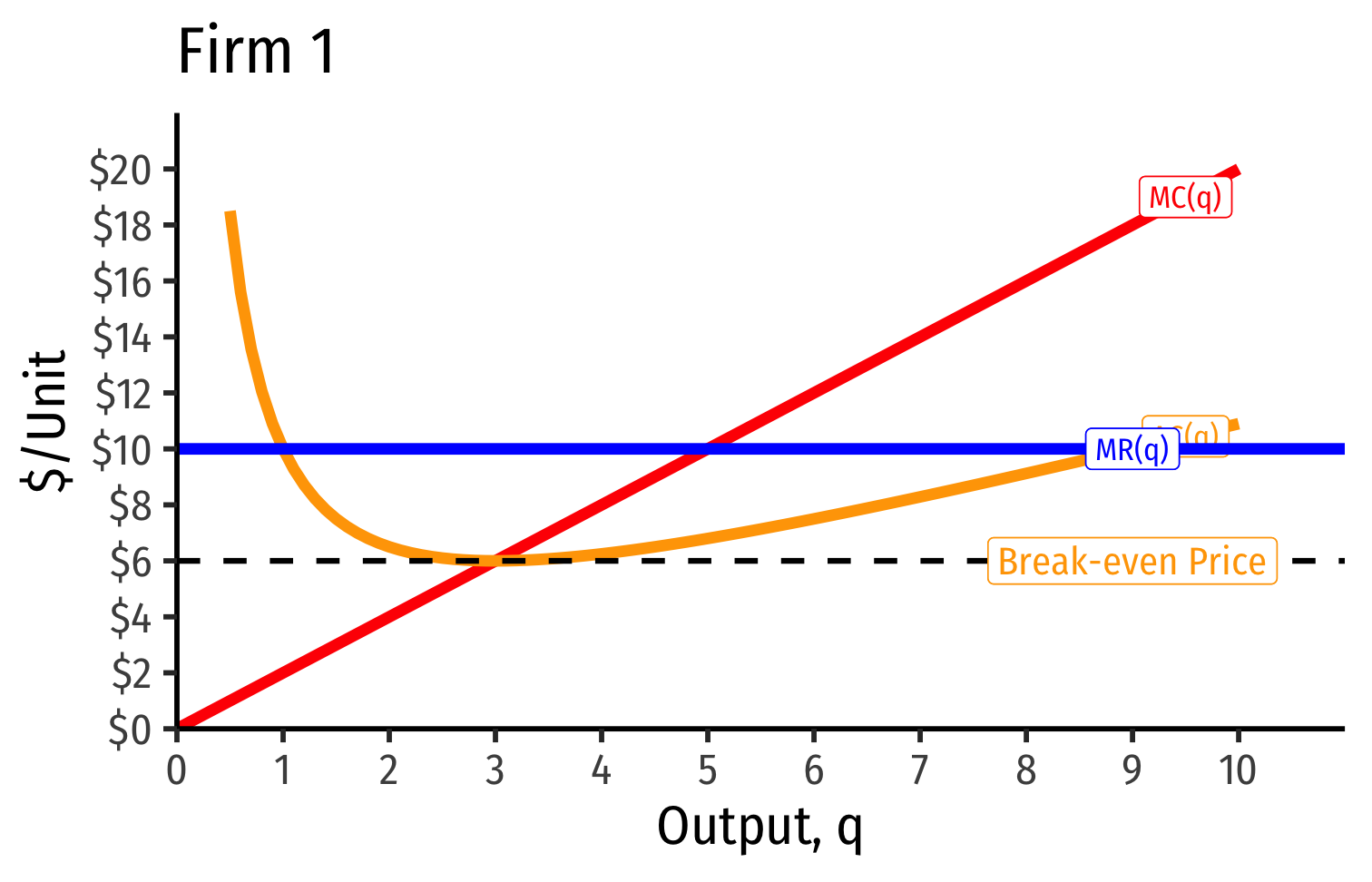
at a market price of $6
- Firm earns “normal” economic profits
At any market price below $6.00, firm earns losses
- Short Run: firm shuts down if
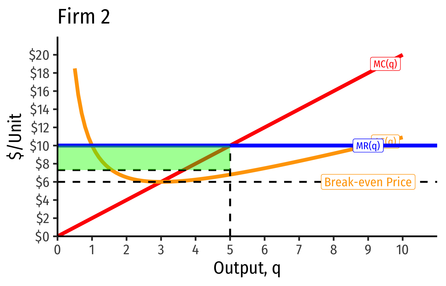
At any market price above $6.00, firm earns “supernormal” profits (>0)
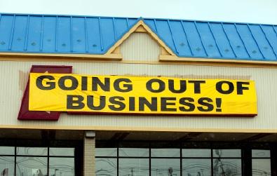
Firm Supply Decisions in the Short Run vs. Long Run
Short run: firms that shut down stuck in market, incur fixed costs
Long run: firms earning losses can exit the market and earn
- No more fixed costs, firms can sell/abandon at
Firm Supply Decisions in the Short Run vs. Long Run
Short run: firms that shut down stuck in market, incur fixed costs
Long run: firms earning losses can exit the market and earn
- No more fixed costs, firms can sell/abandon at
Entrepreneurs not currently in market can enter and produce, if entry would earn them

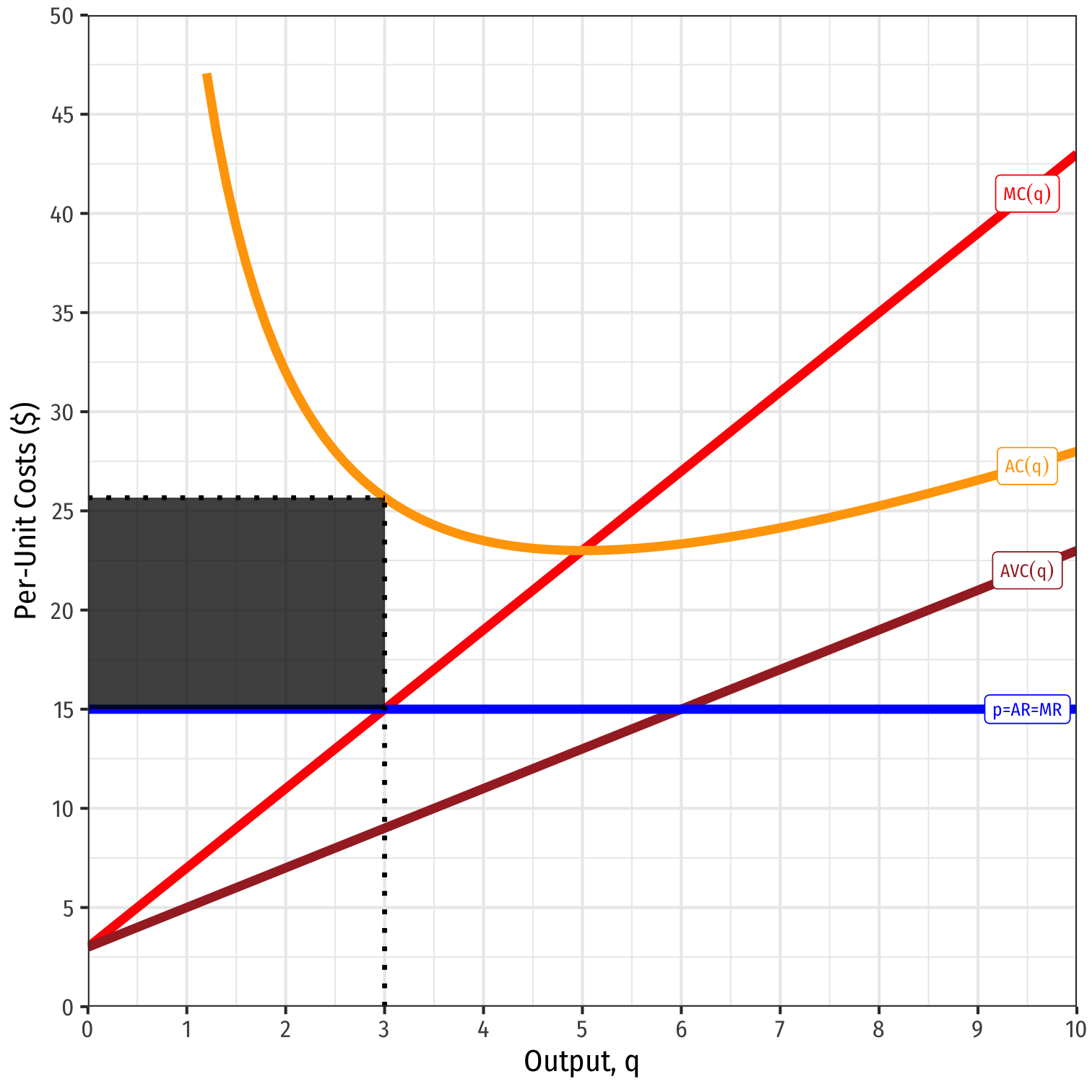
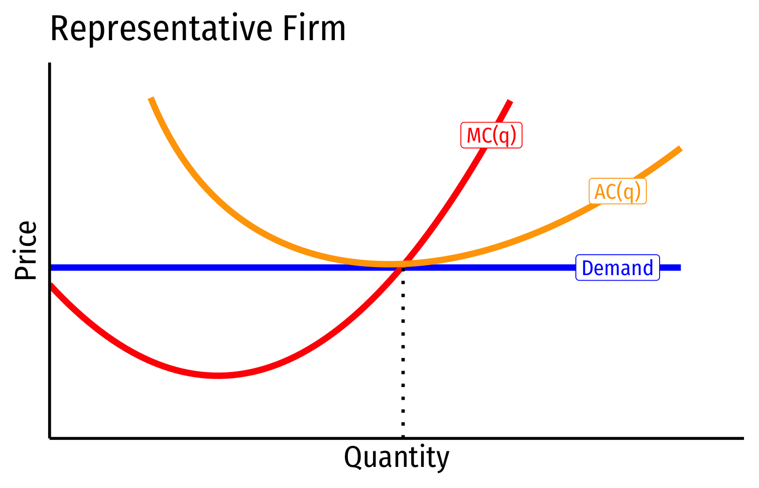
Firm's Long Run Supply: Visualizing
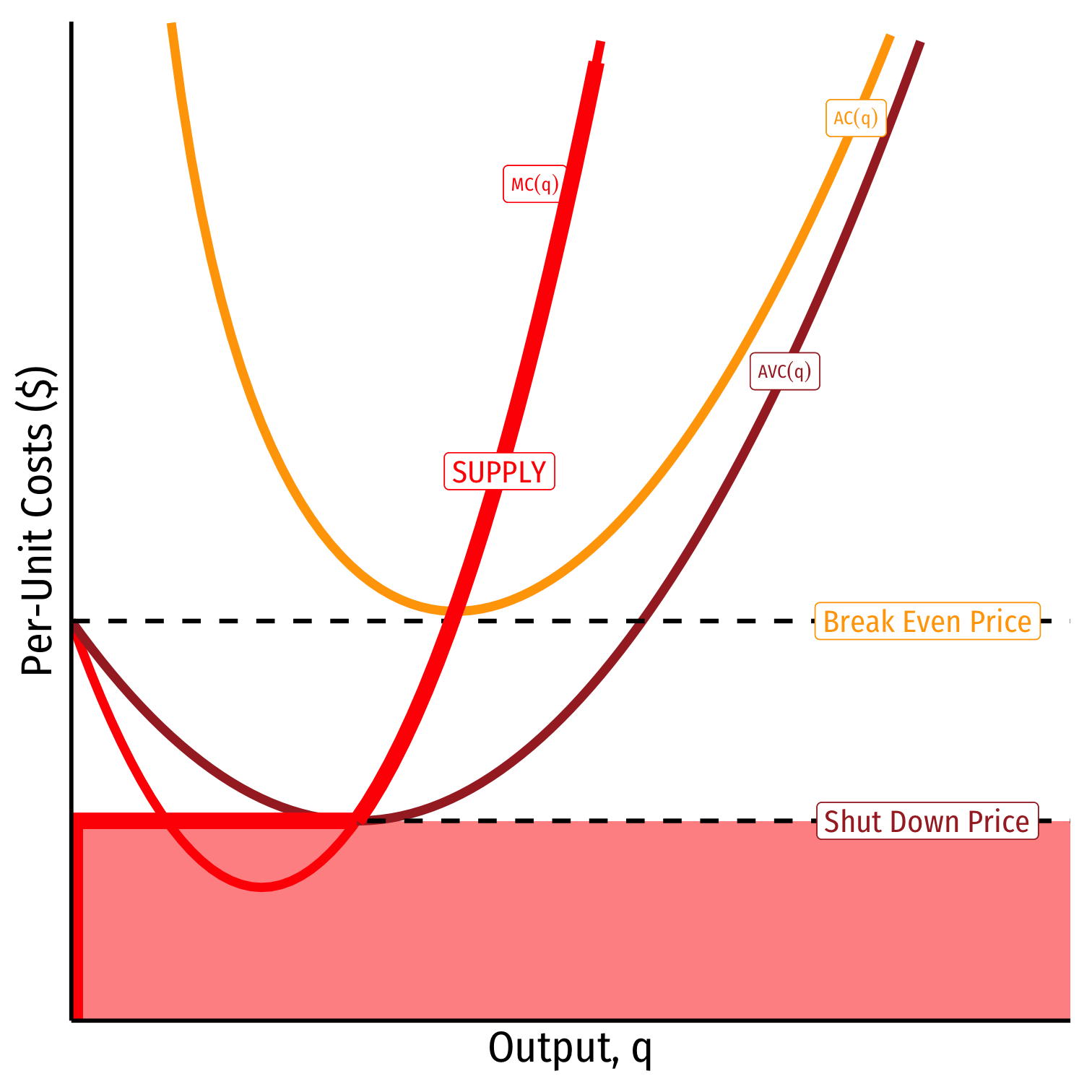
When
Profits are negative
Short run: shut down production
- Firm loses more by producing than by not producing
Long run: firms in industry exit the industry
- No new firms will enter this industry
Firm's Long Run Supply: Visualizing
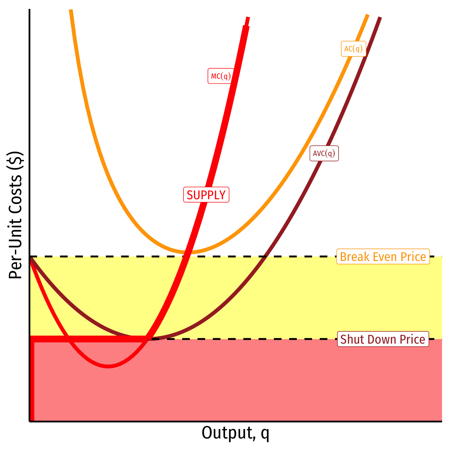
When
Profits are negative
Short run: continue production
- Firm loses less by producing than by not producing
Long run: firms in industry exit the industry
- No new firms will enter this industry
Firm's Long Run Supply: Visualizing
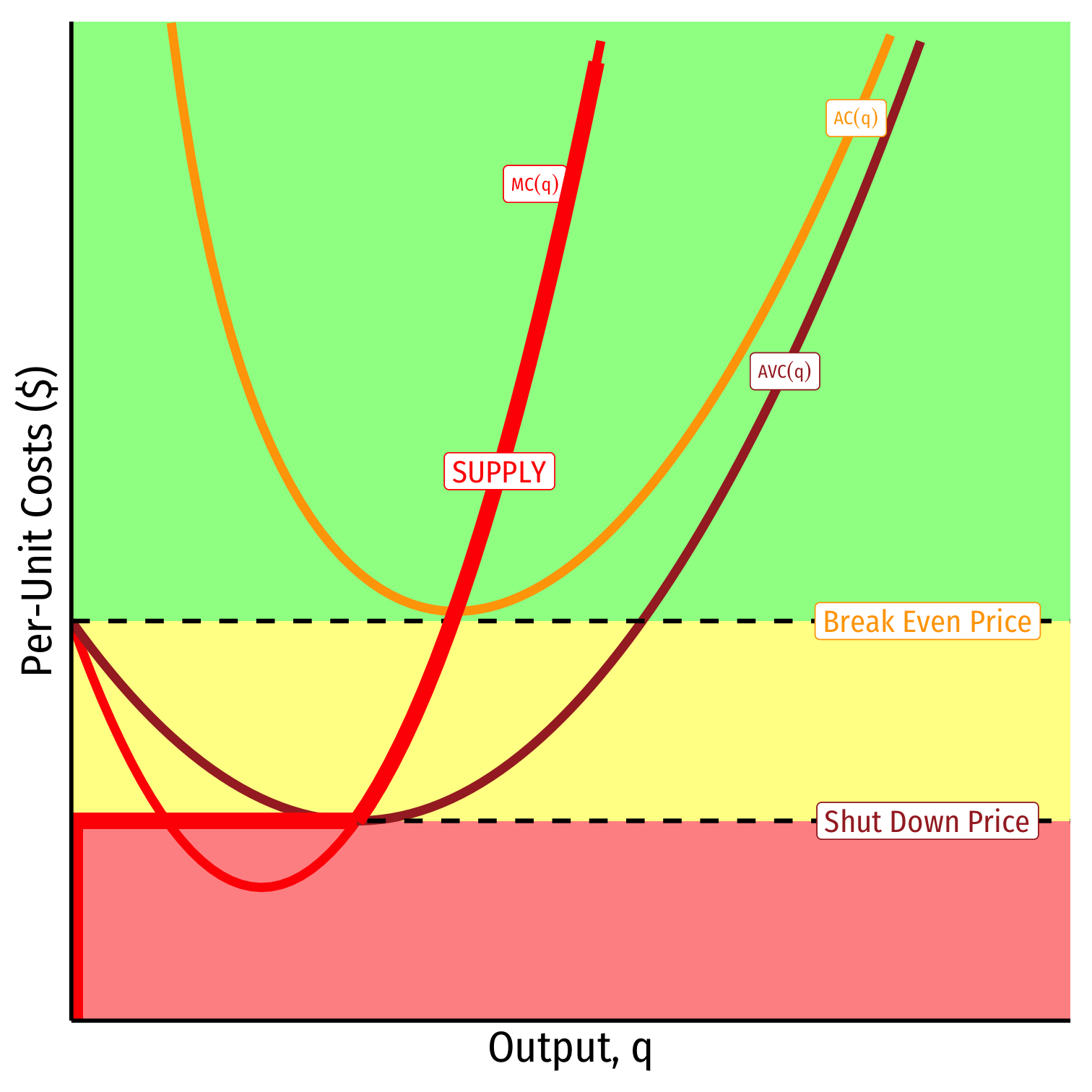
When
Profits are positive
Short run: continue production
- Firm earning profits
Long run: firms in industry stay in industry
- New firms will enter this industry
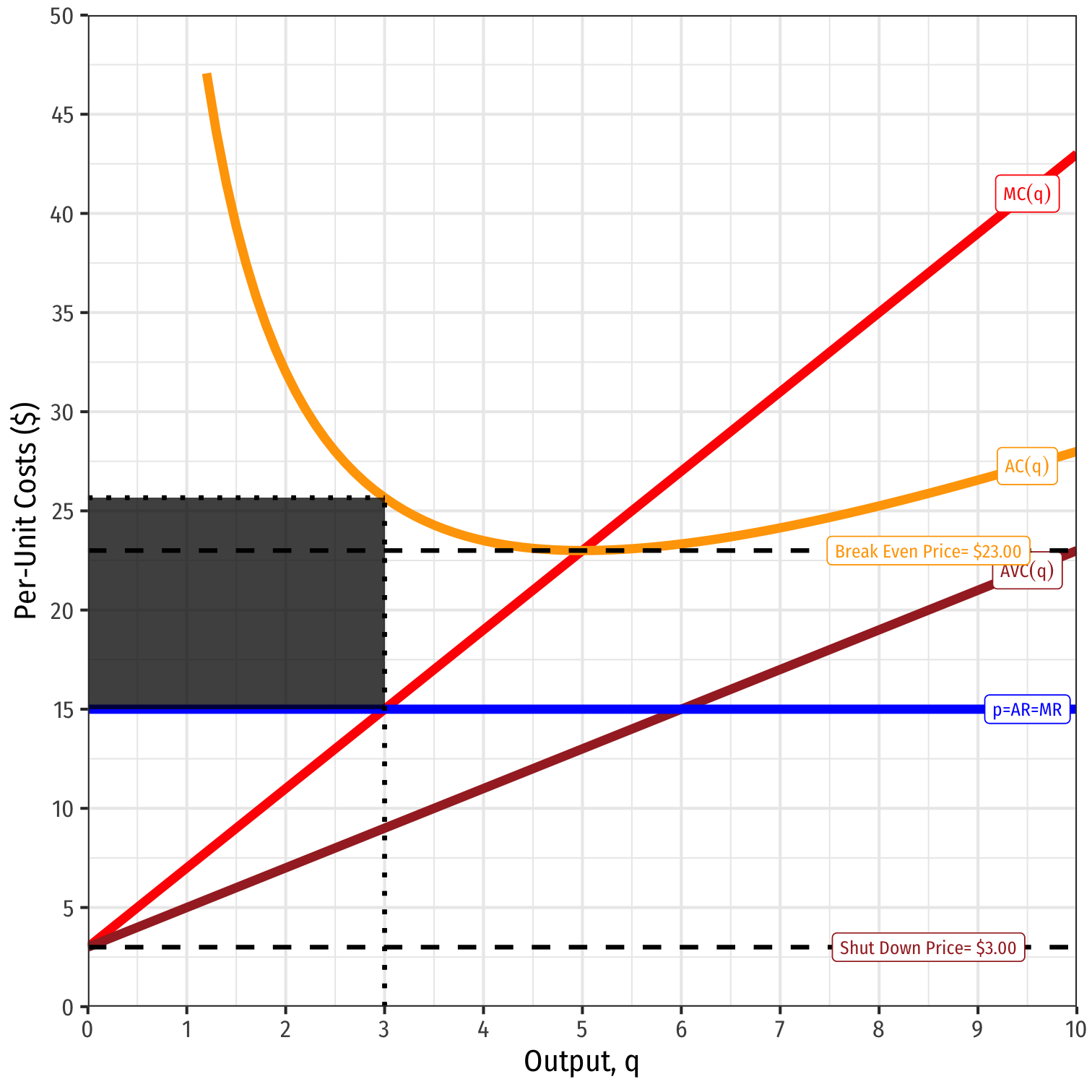
Profit Maximization Rules for Firms:
1. Choose such that
2. Profit
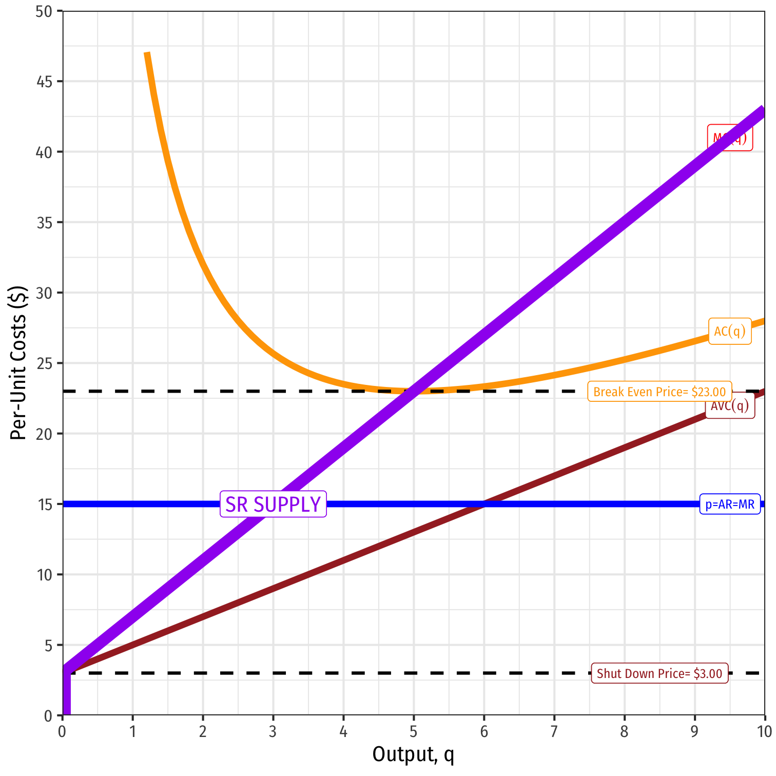
3. Shut down in short run if
Firm’s short run supply curve:
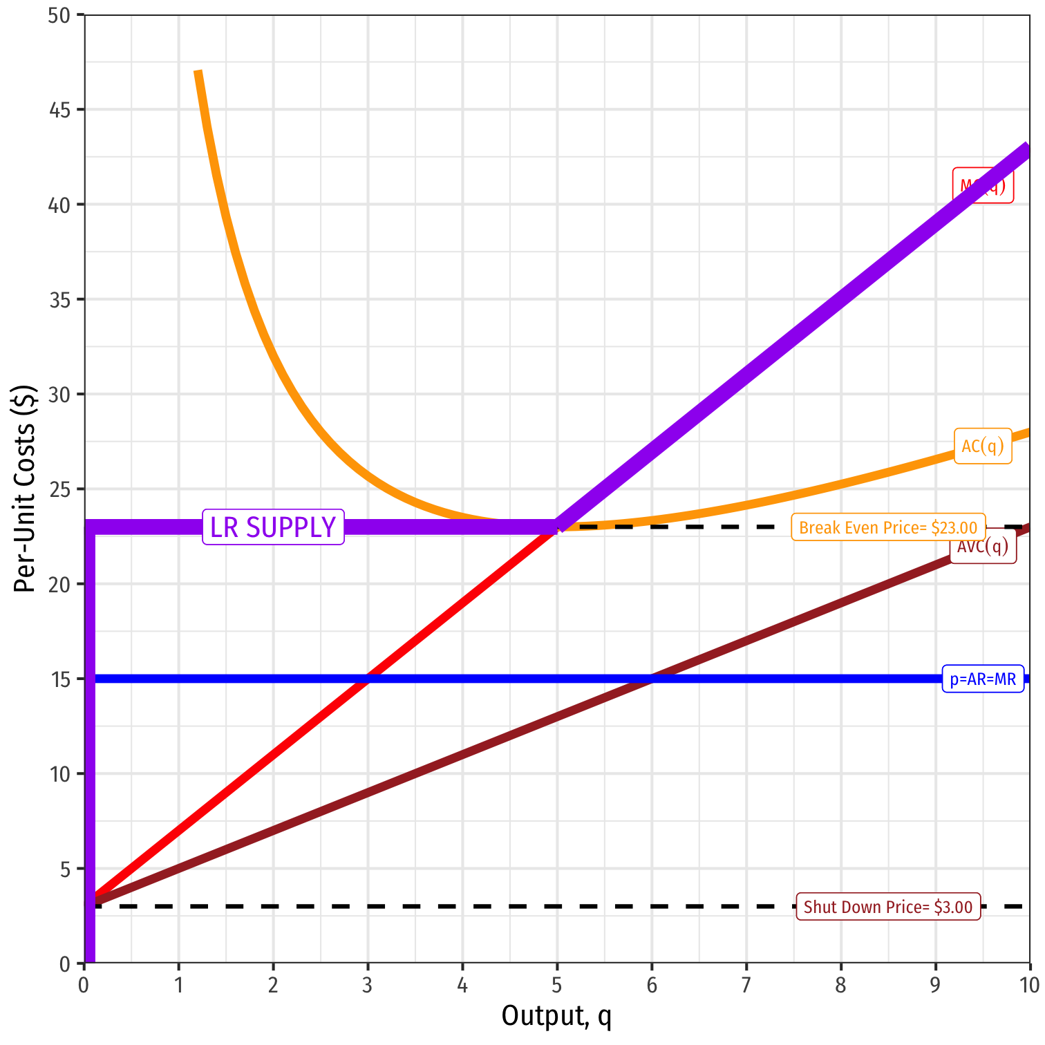
4. Exit in long run if \\(p<AC(q)\\)
Firm’s long run supply curve:

Exit, Entry, and Long Run Industry Equilibrium I
Now we must combine optimizing individual firms with market-wide adjustment to equilibrium
Since , in the long run, profit-seeking firms will:
- Enter markets where
Exit, Entry, and Long Run Industry Equilibrium I
Now we must combine optimizing individual firms with market-wide adjustment to equilibrium
Since , in the long run, profit-seeking firms will:
- Enter markets where
- Exit markets where
Exit, Entry, and Long Run Industry Equilibrium II
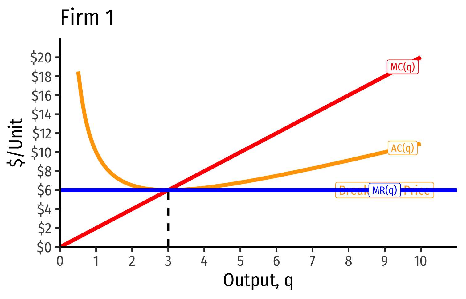
- Long-run equilibrium: entry and exit ceases when for all firms, implying normal economic profits of
Exit, Entry, and Long Run Industry Equilibrium II
Long-run equilibrium: entry and exit ceases when for all firms, implying normal economic profits of
Long run economic profits for all firms in a competitive industry are 0
Firms must earn an accounting profit to stay in business
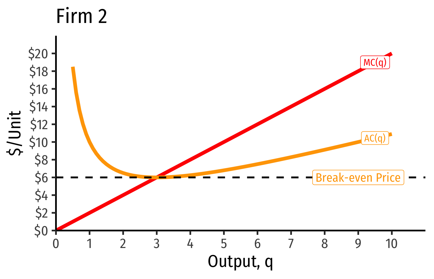
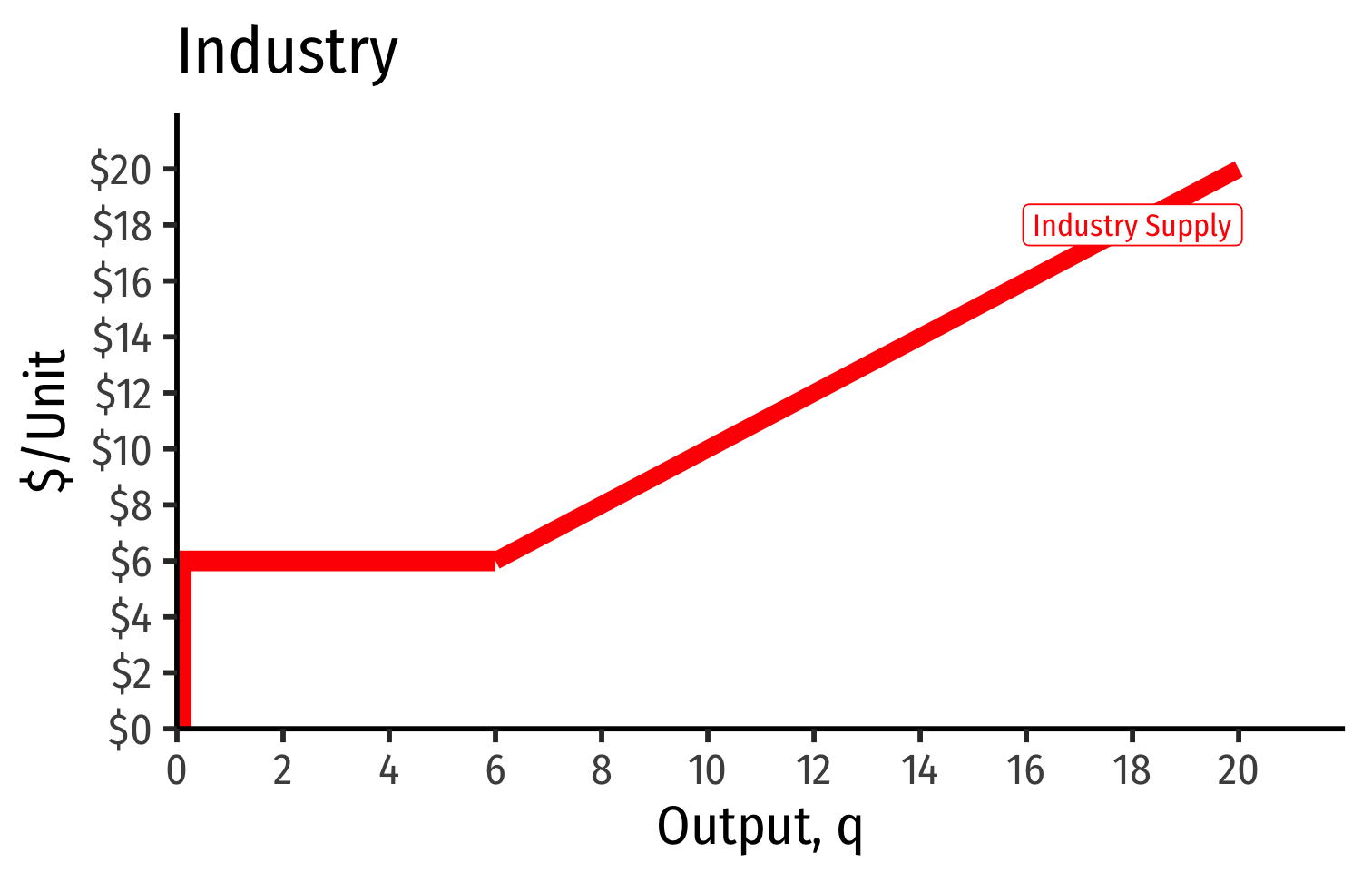
Industry Supply Curves (Identical Firms)

Industry Supply Curves (Identical Firms)
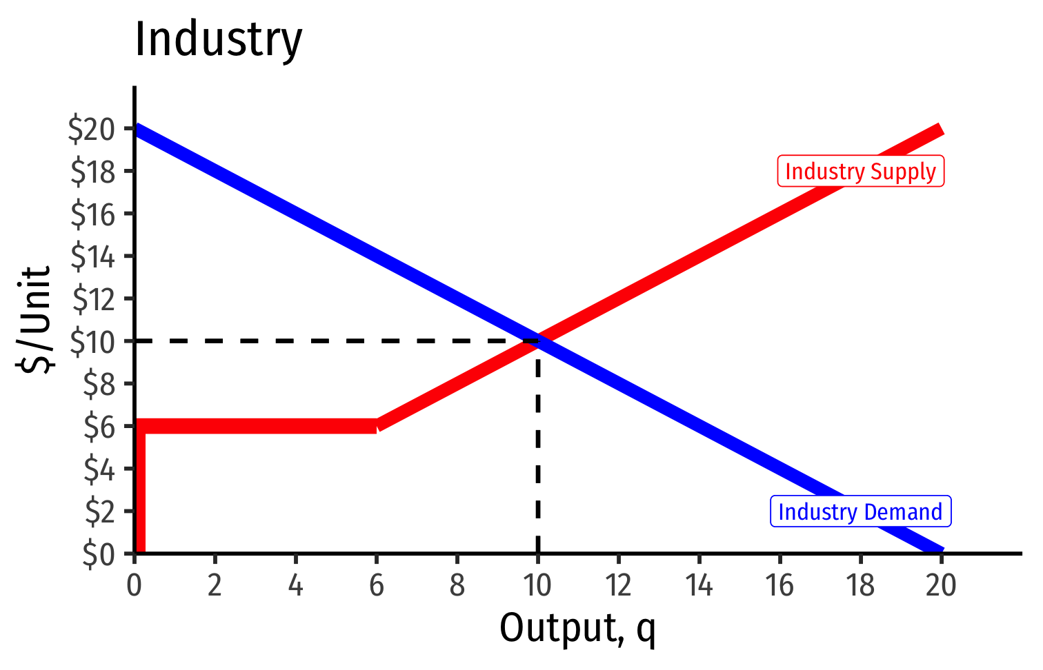
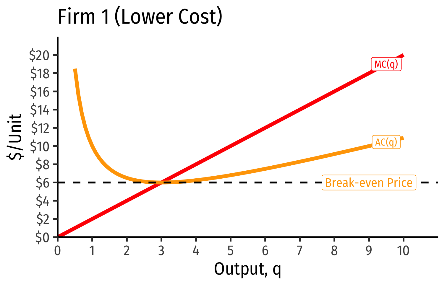
- Industry supply curve is the horizontal sum of all individual firm's supply curves
- Which are each firm's marginal cost curve above its breakeven price
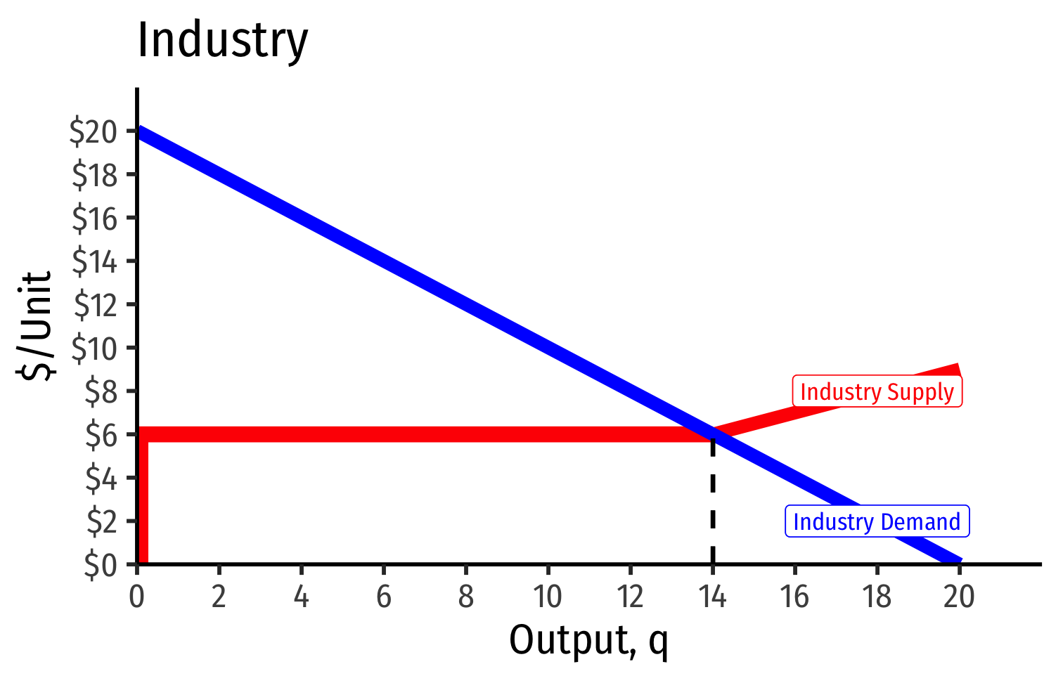
Industry Supply Curves (Identical Firms)


- Industry demand curve (where equal to supply) sets market price, demand for firms
Industry Supply Curves (Identical Firms)

Short Run: each firm is earning profits
Long run: induces entry by firm 3, firm 4, , firm
Industry Supply Curves (Identical Firms)
Short Run: each firm is earning profits
Long run: induces entry by firm 3, firm 4, , firm
- Long run industry equilibrium:
Industry Supply Curves (Identical Firms)
Short Run: each firm is earning profits
Long run: induces entry by firm 3, firm 4, , firm
Long run industry equilibrium: , at $6; supply becomes more elastic
Back to Zero Economic Profits
- Recall, we've essentially defined a firm as a completely replicable recipe (production function) of resources
- “Any idiot” can enter market, buy required at prices , produce at market price and earn the market rate of
Back to Zero Economic Profits
Zero long run economic profit industry disappears, just stops growing
Less attractive to entrepreneurs & start ups to enter than other, more profitable industries
These are mature industries (again, often commodities), the backbone of the economy, just not sexy!

Back to Zero Economic Profits
All factors are paid their market price
- i.e. their opportunity cost — what they could earn elsewhere in economy
Firms earn normal market rate of return
- No excess rewards (economic profits) to attract new resources into the industry, nor losses to push resources out of industry
Back to Zero Economic Profits
But we've so far been imagining a market where every firm is identical, just a recipe “any idiot” can copy
What about if firms have different technologies or costs?
Industry Supply Curves (Different Firms) I
Firms have different technologies/costs due to relative differences in:
- Managerial talent
- Worker talent
- Location
- First-mover advantage
- Technological secrets/IP
- License/permit access
- Political connections
- Lobbying
Let's derive industry supply curve again, and see how this may affect profits

Industry Supply Curves (Different Firms) II
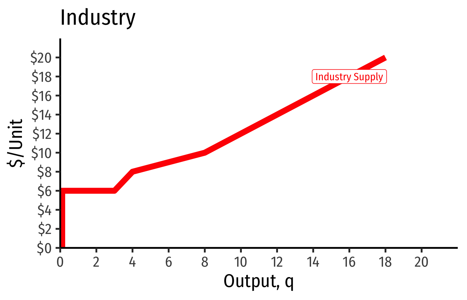
Industry Supply Curves (Different Firms) II
- Industry supply curve is the horizontal sum of all individual firm's supply curves
- Which are each firm's marginal cost curve above its breakeven price
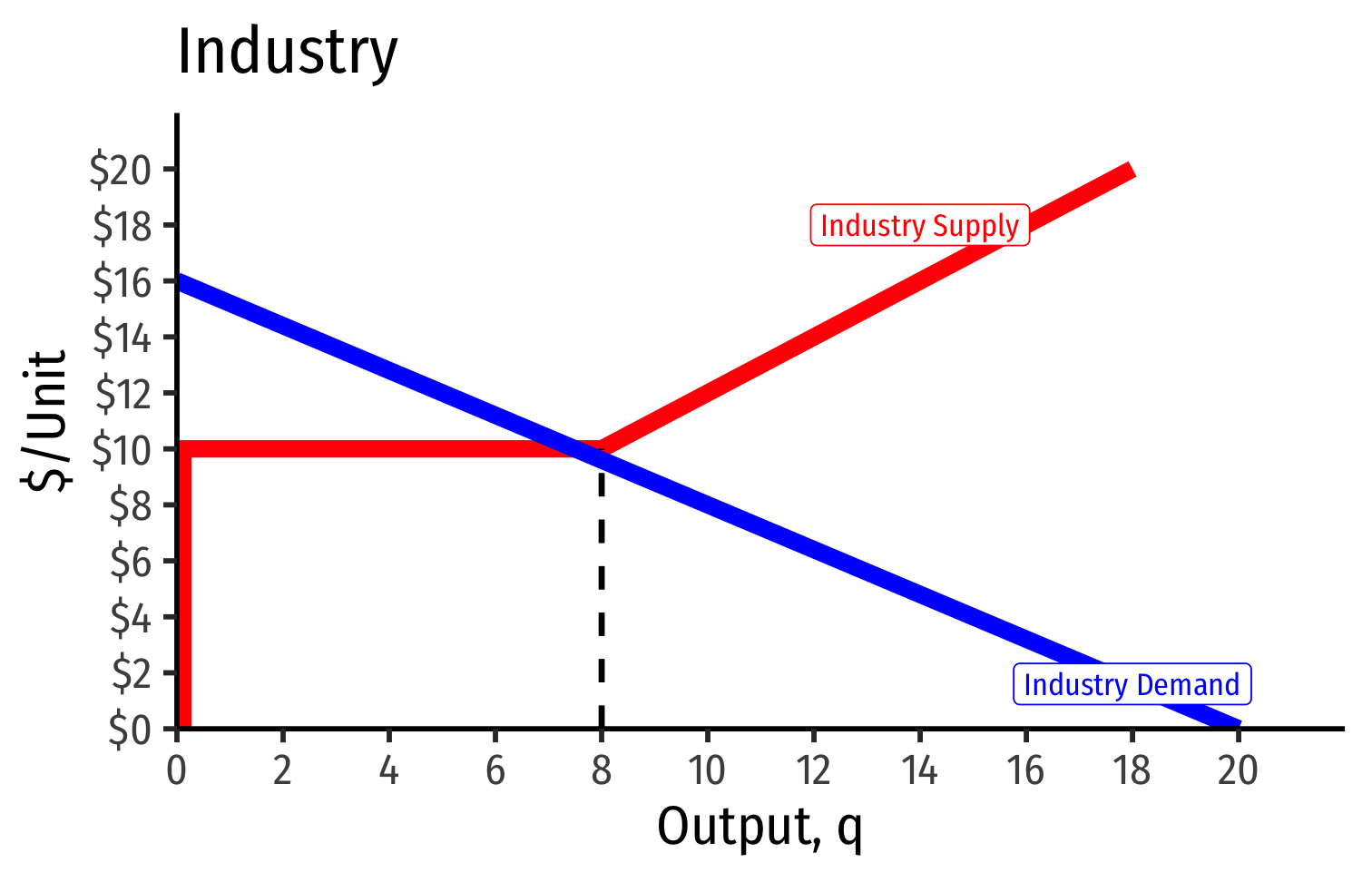
Industry Supply Curves (Different Firms) II


Industry Supply Curves (Different Firms) II
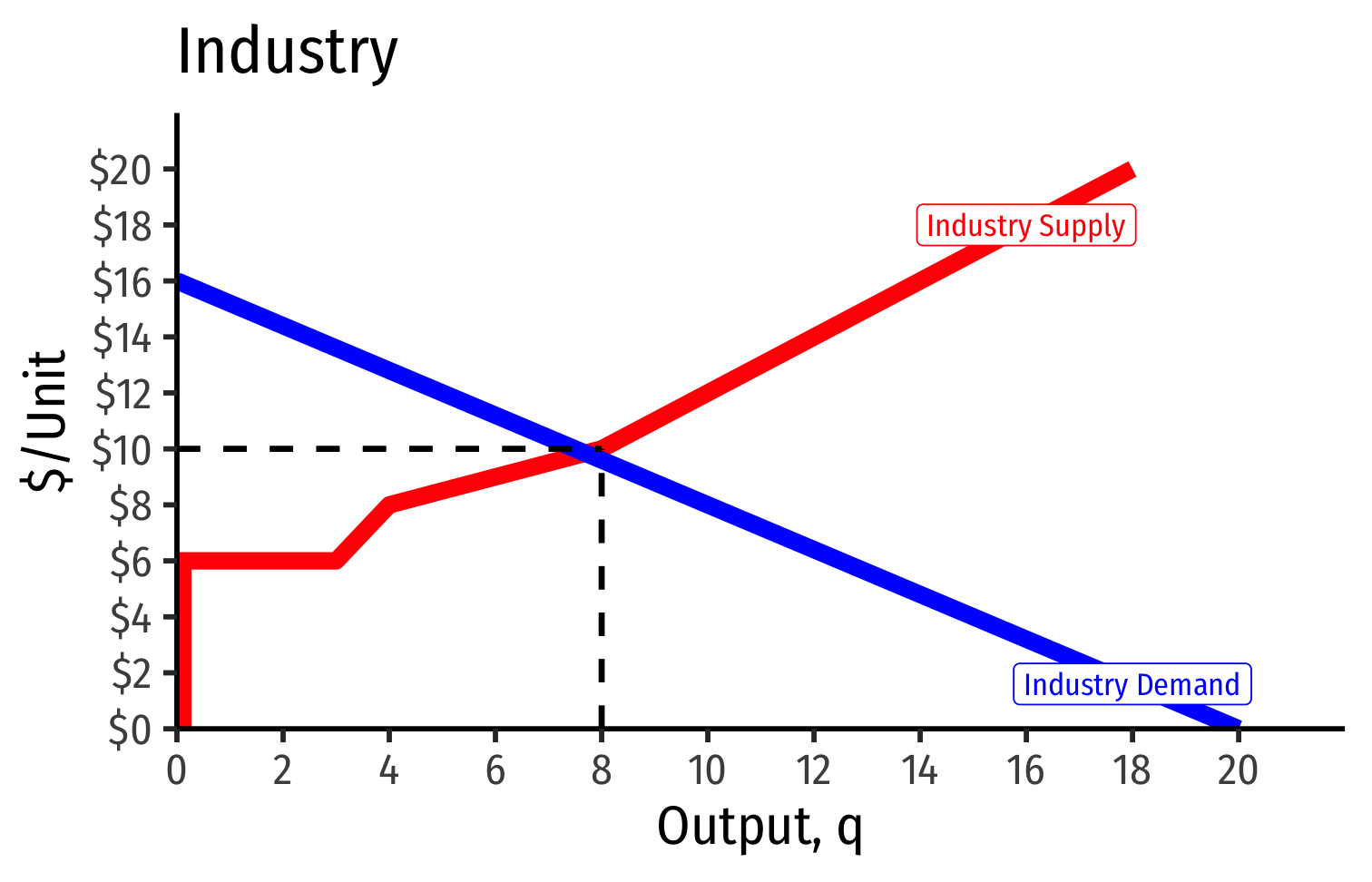
- Industry demand curve (where equal to supply) sets market price, demand for firms
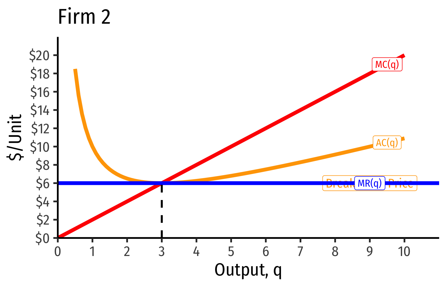
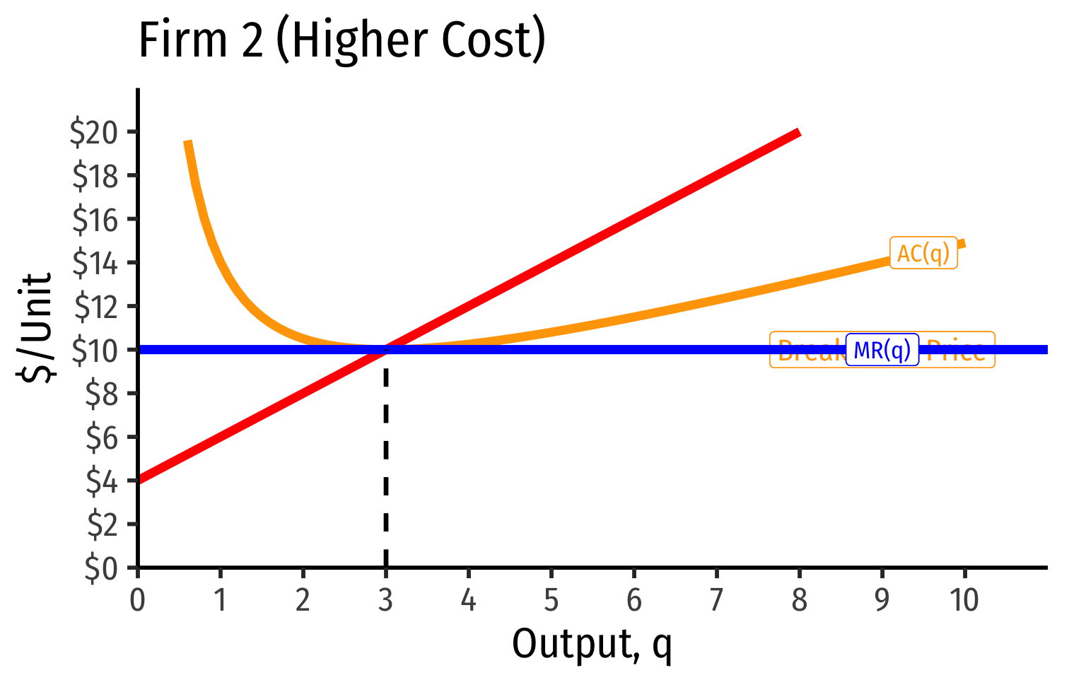
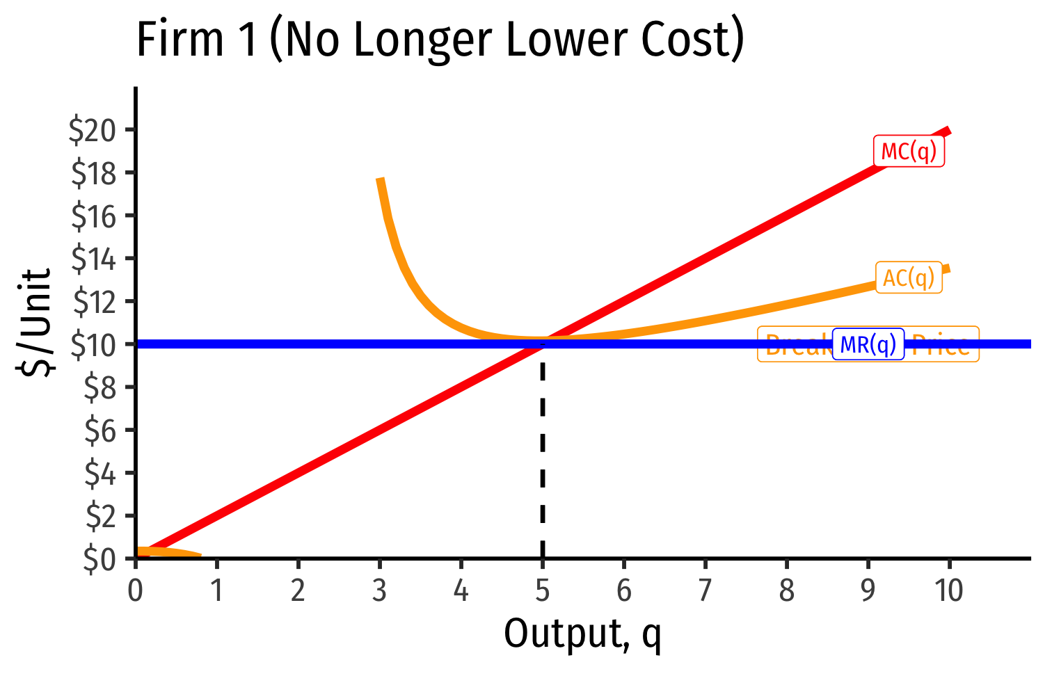
Industry Supply Curves (Different Firms) II
- Industry demand curve (where equal to supply) sets market price, demand for firms
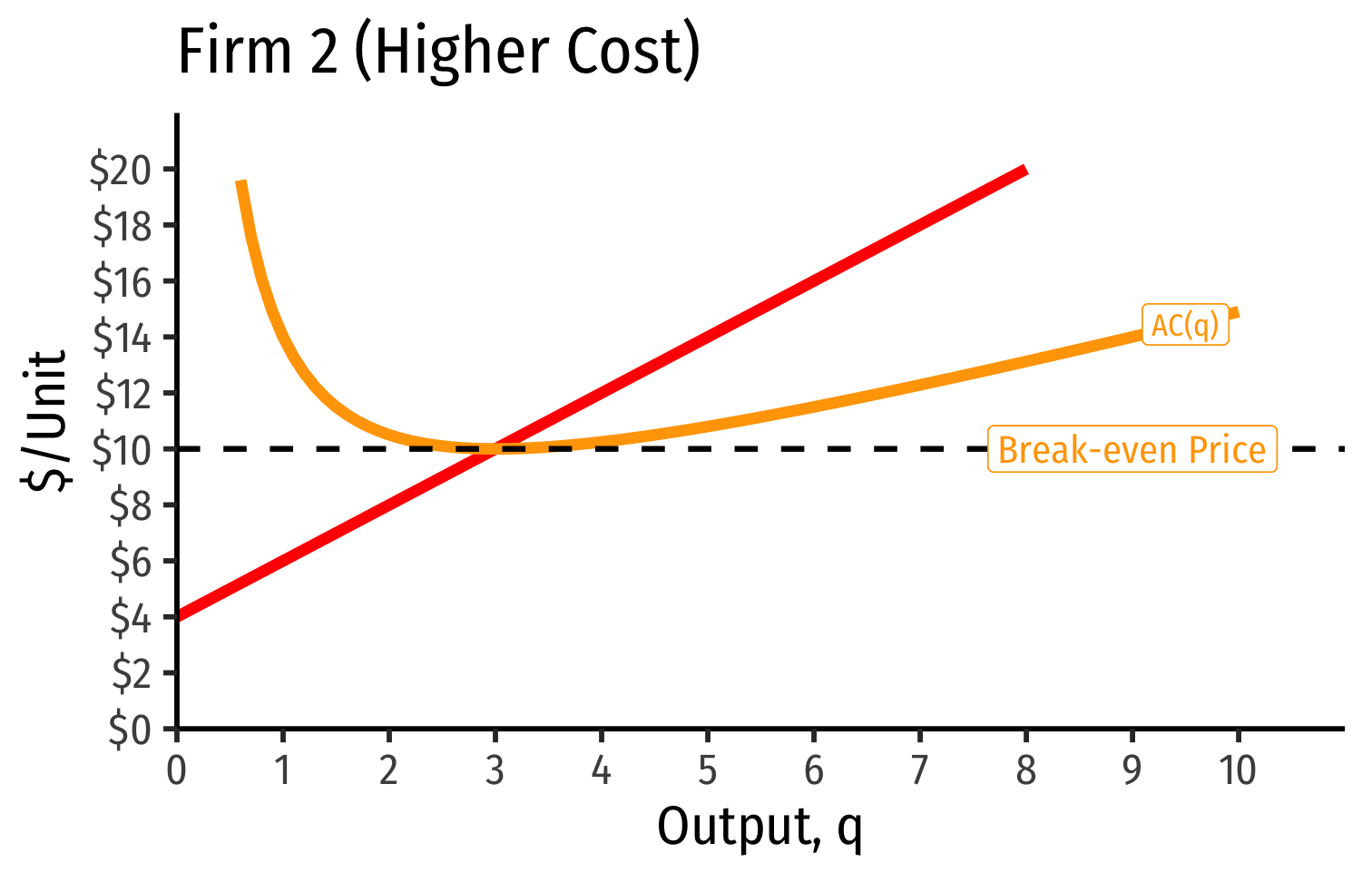
- Long run industry equilibrium: , for marginal (highest cost) firm (Firm 2)
Industry Supply Curves (Different Firms) II
- Industry demand curve (where equal to supply) sets market price, demand for firms
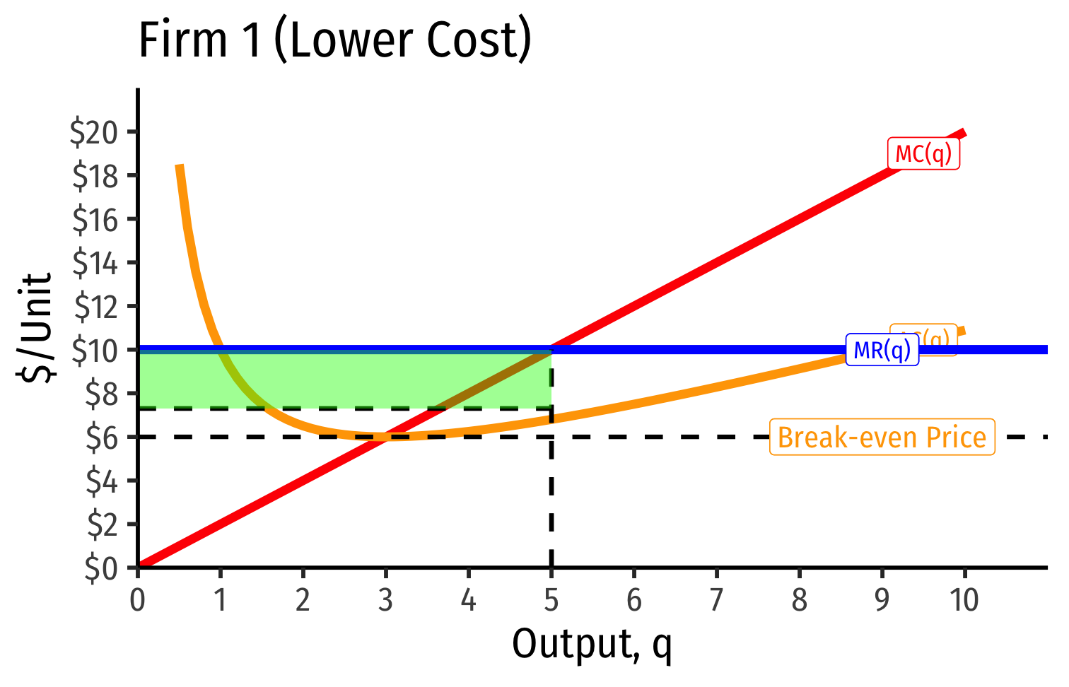
- Long run industry equilibrium: , for marginal (highest cost) firm (Firm 2)
- Firm 1 (lower cost) appears to be earning profits...(we’ll come back to this)
Economic Rents and Zero Economic Profits I

Long-run equilibrium of the marginal (highest-cost) firm
The marginal firm earns normal economic profit (of zero)
- Otherwise, if for that firm, would induce more entry into industry!
Generalized, No-Profitable Entry Condition: in equilibrium, no firm can earn positive profits by entering the industry
Economic Rents and Zero Economic Profits I
“Inframarginal” (lower-cost) firms are using resources that earn economic rents
- returns higher than their opportunity cost (what is needed to bring them into this industry)
Economic rents arise from relative differences between resources
Economic Rent

Economic rent: a return or payment for a resource above its normal market return (opportunity cost)
Has no allocative effect on resources, entirely “inframarginal”
A windfall return that resource owners get for free
Sources of Economic Rents
- Some factors are relatively scarce in the whole economy
- (talent, location, secrets, IP, licenses, being first, political favoritism)
Firms Using Resources with Economic Rents
Inframarginal firms that employ these scarce factors gain a short-run profits from having lower costs/higher productivity
...But what will happen to the prices for their scarce factors over time?
Economic Rents Examples


Economic Rents and Zero Economic Profits
In a competitive market, over the long run, profits are dissipated through competition
- Rival firms willing to pay for the scarce factor to gain an advantage
Competition over acquiring the scarce factors pushes up their prices
- i.e. higher costs to firms of using the factor!
Rents are included in the opportunity cost (price) for inputs over long run
- Must pay a factor enough to keep it out of other uses
Economic Rents and Zero Economic Profits

From the firm’s perspective, over the long-run, rents are included in the price (opportunity cost) of the scarce factor
- Must pay a factor enough to keep it out of other uses
Firm does not earn the rents, they raise firm's costs and squeeze profits to zero!
Economic Rents Reduce Firms’ Profits Over Long Run

- Short Run: firm that possesses scarce rent-generating factors has lower costs, perhaps short-run profits
Economic Rents Reduce Firms’ Profits Over Long Run

Short Run: firm that possesses scarce rent-generating factors has lower costs, perhaps short-run profits
Long run: competition over those factors pushes up their prices, raising costs to firm, until its profits go to zero as well
- Increase in fixed cost (scarce factor), raising AC(q), which now includes rents (more info in appendix)
Economic Rents Go To Resource Owners

Owners of scarce factors (workers, landowners, inventors, etc) earn the rents as higher income for their services (wages, land rent, interest, royalties, etc).
Often induces competition to supply alternative factors, which may dissipate the rents (to zero)
- More workers invest in becoming talented, try to create new inventions, build new land, etc.
Recall: Accounting vs. Economic Point of View
Recall “economic point of view”:
Producing your product pulls scarce resources out of other productive uses in the economy
Profits attract resources: pulled out of other (less valuable) uses
Losses repel resources: pulled away to other (more valuable) uses
Zero profits keep resources where they are
- Implies society is using resources optimally


Example: Visualized
Example: Visualized
Example: Visualized
Example: Visualized
Example: Visualized
Perfectly Competitive Market
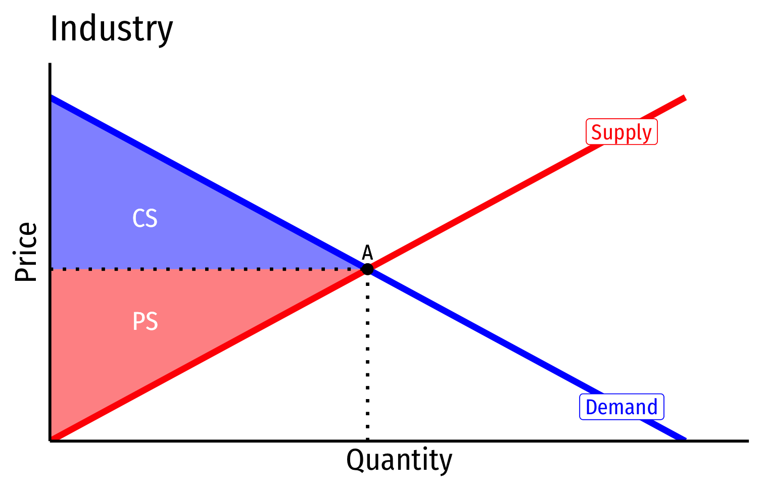
- In a competitive market in long run equilibrium:
- Economic profit is driven to $0; resources (factors of production) optimally allocated
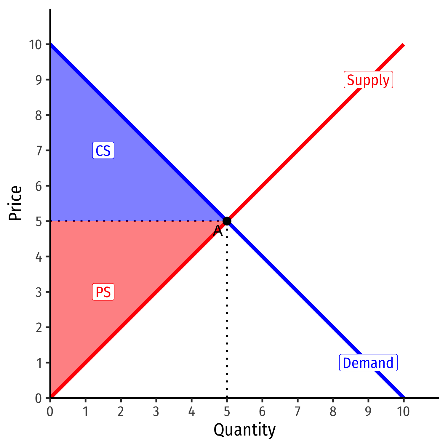
- Allocatively efficient: , maximized CS PS
- Productively efficient: (otherwise firms would enter/exit)
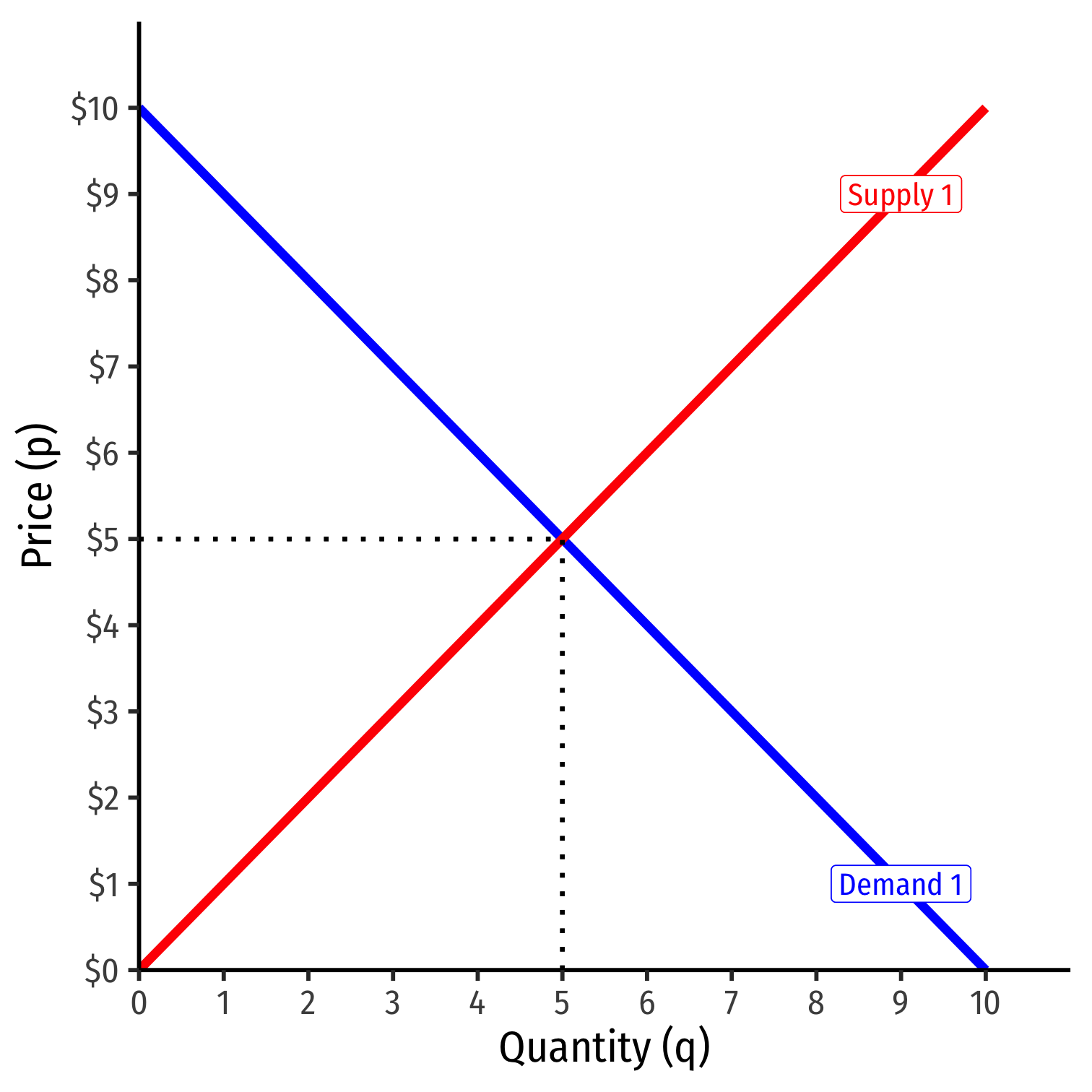
Market-Clearing Prices
- Supply and demand set the market-clearing price for all units exchanged (bought and sold)
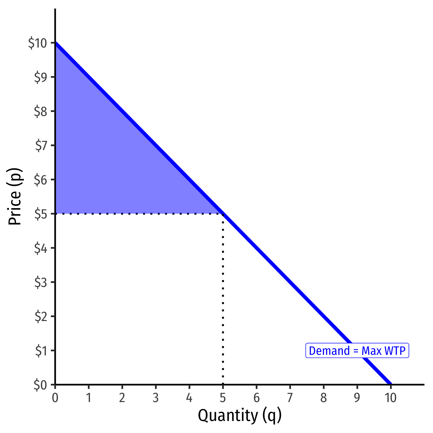
Consumer Surplus I
Demand function measures how much you would hypothetically be willing to pay for various quantities
- "reservation price"
You often actually pay (the market-clearing price, a lot less than your reservation price
The difference is consumer surplus

Consumer Surplus II
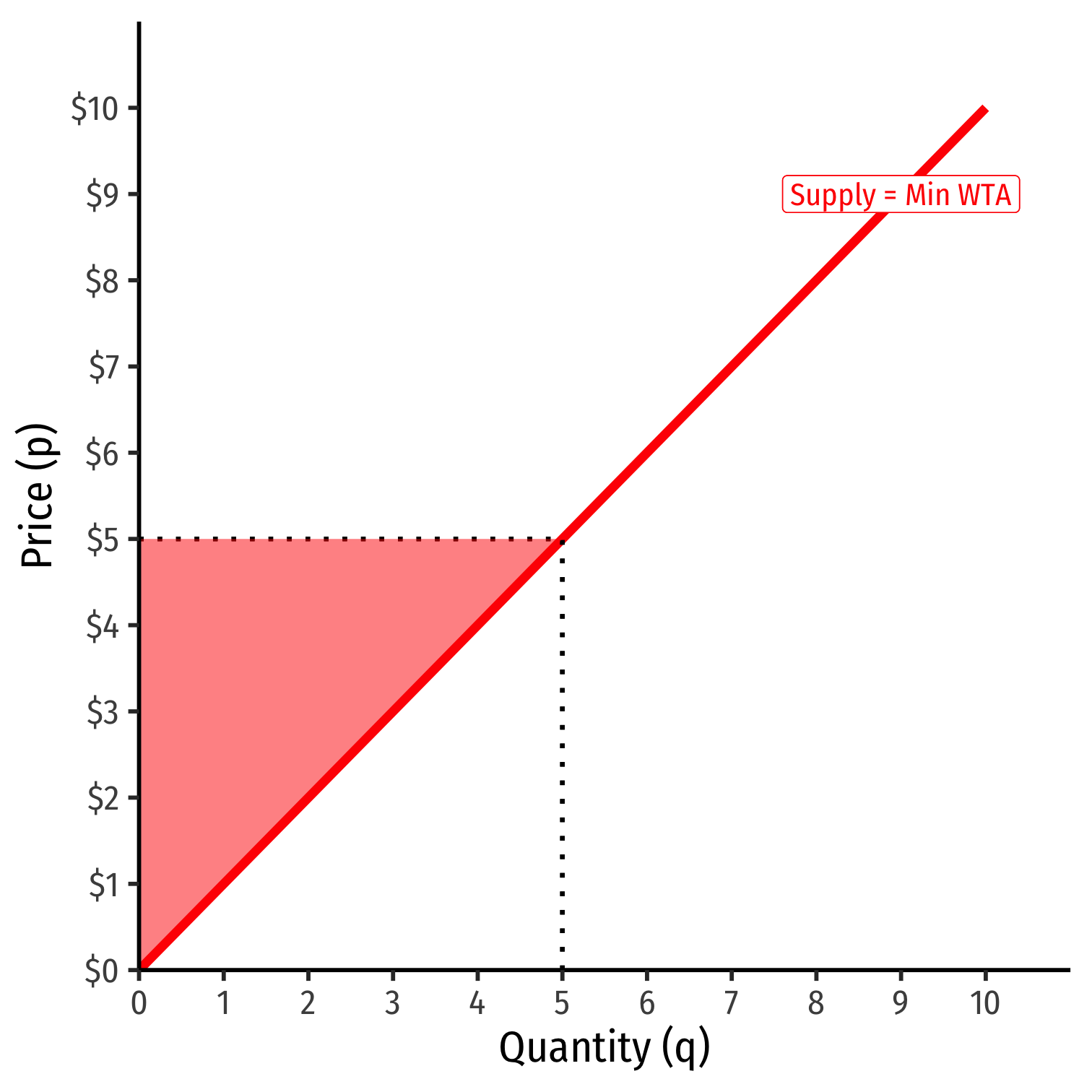
Producer Surplus I
Supply function measures how much you would hypothetically be willing to accept to sell various quantities
- "reservation price"
You often actually receive (the market-clearing price, a lot more than your reservation price
The difference is producer surplus
Market Efficiency in Competitive Equilibrium I
Allocative efficiency: resources are allocated to highest-valued uses
- Goods produced up to the point where
All potential gains from trade are fully exhausted
Market Efficiency in Competitive Equilibrium II
Economic surplus = Consumer surplus + Producer surplus
Maximized in competitive equilibrium
Resources flow away from those who value them the lowest to those that value them the highest
The social value of resources is maximized by allocating them to their highest valued uses!
