1.8 — Factor Markets

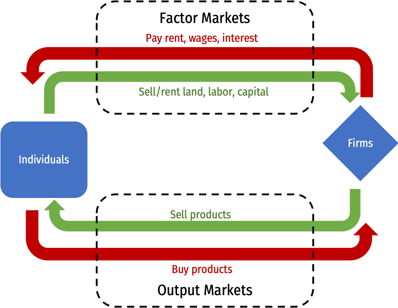
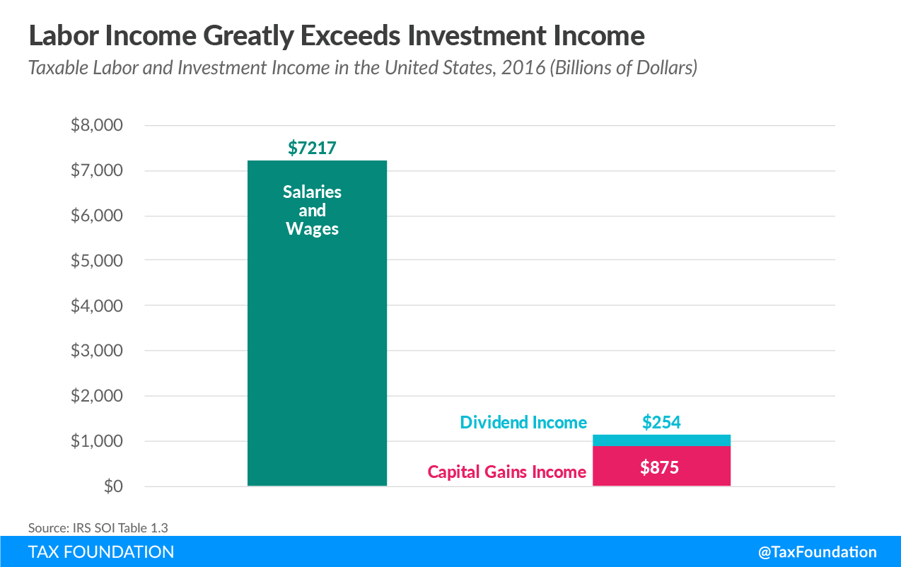
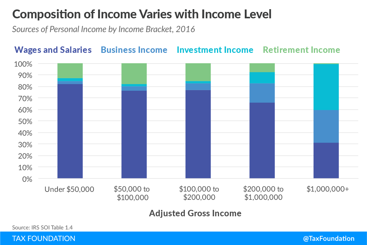
# 1.8 — Factor Markets

## ECON 326 • Industrial Organization • Spring 2023

### Ryan Safner<br> Associate Professor of Economics <br> <a href="mailto:safner@hood.edu"><i class="fa fa-paper-plane fa-fw"></i>safner@hood.edu</a> <br> <a href="https://github.com/ryansafner/ioS23"><i class="fa fa-github fa-fw"></i>ryansafner/ioS23</a><br> <a href="https://ioS23.classes.ryansafner.com"> <i class="fa fa-globe fa-fw"></i>ioS23.classes.ryansafner.com</a><br>

---
class: inverse

# Outline

### [Labor Supply Decisions](#12)

### [Labor Market for Competitive Firm](18)

### [Labor Market for a Monopoly](#33)

### [Monopsony Power](#37)

### [Monopoly Power in Labor Markets: Unions](#59)

---

# Returning to Firms

.pull-left[
- Recall a firm uses technology that buys inputs, transforms them, and sells output
`$$q=f(k,l)$$`
  - We classified inputs into the .hi[factors of production]: land, labor, capital

- We *assumed* fixed factor prices
  - show up in total cost `$=wL+rK$`

- Where do they come from? .hi[Factor markets]
]

---

# Circular Flow

---

# Firms’ Payments to Factors are Income To Households

.quitesmall[
<table>
 <thead>
  <tr>
   <th style="text-align:left;"> Income Type </th>
   <th style="text-align:right;"> Amount (2016) </th>
   <th style="text-align:right;"> Percent </th>
  </tr>
 </thead>
<tbody>
  <tr>
   <td style="text-align:left;"> Salaries and wages </td>
   <td style="text-align:right;"> $7217 Bn </td>
   <td style="text-align:right;"> 68.45% </td>
  </tr>
  <tr>
   <td style="text-align:left;"> Taxable pensions and annuities </td>
   <td style="text-align:right;"> $694 Bn </td>
   <td style="text-align:right;"> 6.58% </td>
  </tr>
  <tr>
   <td style="text-align:left;"> Partnership and S corporation net income </td>
   <td style="text-align:right;"> $629 Bn </td>
   <td style="text-align:right;"> 5.97% </td>
  </tr>
  <tr>
   <td style="text-align:left;"> Capital gains less losses </td>
   <td style="text-align:right;"> $621 Bn </td>
   <td style="text-align:right;"> 5.89% </td>
  </tr>
  <tr>
   <td style="text-align:left;"> Business net income </td>
   <td style="text-align:right;"> $389 Bn </td>
   <td style="text-align:right;"> 3.69% </td>
  </tr>
  <tr>
   <td style="text-align:left;"> Taxable Social Security benefits </td>
   <td style="text-align:right;"> $286 Bn </td>
   <td style="text-align:right;"> 2.71% </td>
  </tr>
  <tr>
   <td style="text-align:left;"> Taxable IRA distributions </td>
   <td style="text-align:right;"> $258 Bn </td>
   <td style="text-align:right;"> 2.45% </td>
  </tr>
  <tr>
   <td style="text-align:left;"> Ordinary dividends </td>
   <td style="text-align:right;"> $254 Bn </td>
   <td style="text-align:right;"> 2.41% </td>
  </tr>
  <tr>
   <td style="text-align:left;"> Total rental and royalty net income </td>
   <td style="text-align:right;"> $98 Bn </td>
   <td style="text-align:right;"> 0.93% </td>
  </tr>
  <tr>
   <td style="text-align:left;"> Taxable interest </td>
   <td style="text-align:right;"> $97 Bn </td>
   <td style="text-align:right;"> 0.92% </td>
  </tr>
</tbody>
</table>
]

---

# Firms’ Payments to Factors are Income To Households

---

# Supply and Demand in Factor Markets

- The price of a factor is governed by the same market forces as output:

- .hi-red[Supply of Factor]: willingness of factor owners to accept and sell/rent their services to firms
  - landowners, workers, capitalists, resource owners, suppliers

- .hi-blue[Demand for Factor]: willingness of firms to pay for/hire factor services
]

.pull-right[
<img src="1.8-slides_files/figure-html/unnamed-chunk-2-1.png" width="504" style="display: block; margin: auto;" />
]

---

# Factor Market Prices and Opportunity Costs

- .hi[Factor price represents **opportunity cost** of hiring a factor for an alternative use]
  - Firms not only pay for direct use of a factor, but also indirectly for *not using* it in an alternate process!

]

# Factor Market Prices and Opportunity Costs

- .green[**Example**]: a producer of hammers buys steel, pays (the opportunity cost) for "taking" the steel away from alternative uses

]

---

# Factor Market Prices and Opportunity Costs

- .green[**Example**]: e.g. salary for a skilled worker must be high enough to keep them at their current firm, and not be attracted to other firms/industries

]

---

# Example Factor Market: Labor Markets

- We’ll focus just on the .hi[market for labor] as an example factor market

- Can do the same for *any* factor market 
  - (e.g. capital, land, materials, etc.)
]

---

# Labor Supply Decisions

---

# Labor Supply Decisions

- The .red[Supply of Labor] comes from **individual decisions to work**

- Labor is considered a .hi[disutility] (a .hi[bad])
  - **Opportunity cost** of labor is .hi[leisure]
  - But, labor generates .hi-purple[income] for .hi-purple[consumption] (a good)

- Tradeoff: if you work more, you get more income, but less leisure
]

![:scale 50%](../images/freedom.jpg)
]
]

---

# Modeling Labor Supply Decisions: A Change In Wages

- We often see “backward-bending” labor supply curves

- Depends on whether income or substitution effect dominates
]
.pull-right[
<img src="1.8-slides_files/figure-html/unnamed-chunk-3-1.png" width="504" style="display: block; margin: auto;" />

]

---

# A Brief Digression on Economic Rents I

- Recall .hi-red[market supply] is the **minimum willingness to accept**, the minimum price necessary to bring a resource to market (its opportunity cost)

- But all (equivalent) labor is paid the *market wage*, `$w^*$` determined by market labor supply and labor demand

]

<img src="1.8-slides_files/figure-html/unnamed-chunk-4-1.png" width="504" style="display: block; margin: auto;" />
]

---

# A Brief Digression on Economic Rents II

- Some workers would have accepted a job for less than `$w^*$`

- These inframarginal workers earn .hi[economic rent] in excess of what is needed to bring them into the market (their opportunity cost)

]

<img src="1.8-slides_files/figure-html/unnamed-chunk-5-1.png" width="504" style="display: block; margin: auto;" />
]

---

# A Brief Digression on Economic Rents III

- Consider a factor (such as land) for which the supply is perfectly inelastic (e.g. a fixed supply)

- Then the **entire value of the land is economic rent**!

- .hi-purple[The *less* elastic the supply of a factor, the *more* economic rent it generates!]

]

<img src="1.8-slides_files/figure-html/unnamed-chunk-6-1.png" width="504" style="display: block; margin: auto;" />
]

---

# Labor Market for a Competitive Firm

---

# Derived Demand in Factor Markets

.pull-left[
- Demand for factors is a .hi-purple[“derived demand”]:
  - Firm only demands inputs to the extent they **contribute to producing sellable output**

- Firm faces a .hi-purple[tradeoff] when **hiring more labor**, as more labor `$\Delta L$` creates:
  1. .hi[Marginal Benefit]: Increases output and thus revenue
  2. .hi[Marginal Cost]: Increases costs
]

---

# Marginal Revenue Product (of Labor)

- Hiring more labor increases new output (i.e. labor's .hi-purple[`\$MP_L\$`])
  - [Recall](https://ios23.classes.ryansafner.com/content/1.2-content/): `$MP_L=\frac{\Delta q}{\Delta L}$`, where `$q$` is units of output

- Additional output generates new revenues (i.e. labor's .hi-purple[`\$MR(q)\$`])
  - Recall: `$MR(q)=\frac{\Delta R(q)}{\Delta q}$`, where `$R(q)$` is total revenue
--

- Hiring more labor, on the **margin**, generates a **benefit**, called the .hi-blue[marginal revenue product of labor, `\$MRP_L\$`]:
`$$MRP_L=MP_L* MR(q)$$`
  - i.e. the number of new products a new worker makes times the revenue earned by selling the new products

---

# Marginal Revenue Product for *Competitive* Firms

- This is the .hi-blue[Firm's Demand for Labor]:

`$$MRP_L=MP_L* MR(q)$$`

- For a firm in a .hi[competitive (output) market], firm's `$MR(q)=p$`, hence:

`$$MRP_L=MP_L*p$$`
where `$p$` is the price of the firm's *output*

]

---

# Marginal Revenue Product for *Competitive* Firms

`$$MRP_L=MP_L* p$$`

- Marginal benefit of hiring labor, `$MRP_L$` **falls** with more labor used
    - production exhibits **diminishing marginal returns to labor**!

- .hi[Choke price for labor demand]: price too high for firm to purchase any labor

]

---

# A Competitive *Factor* Market

.pull-left[
<img src="1.8-slides_files/figure-html/unnamed-chunk-9-1.png" width="504" style="display: block; margin: auto;" />
]

.pull-right[
<img src="1.8-slides_files/figure-html/unnamed-chunk-10-1.png" width="504" style="display: block; margin: auto;" />
]

- If the .hi[*factor* market is competitive], labor supply available to an individual firm is *perfectly elastic* at the market price of labor `$(w^*)$`

---