2.3 — Bertrand Competition

# 2.3 — Bertrand Competition

## ECON 326 • Industrial Organization • Spring 2023

### Ryan Safner Associate Professor of Economics <a href="mailto:safner@hood.edu">safner@hood.edu</a> <a href="https://github.com/ryansafner/ioS23">ryansafner/ioS23</a> <a href="https://ioS23.classes.ryansafner.com"> ioS23.classes.ryansafner.com</a>

---

# Bertrand Competition: Moblab

---

# Bertrand Competition: Moblab

- You will be put into a market with one other player

- Each term, both of you simultaneously choose your price

- Firm(s) choosing the lowest price get **all** the customers

]

]

---
# Bertrand Competition: Moblab

- The lowest price `$p_L$` determines the market demand
`$$q=3600-200p_L$$`

- Both firms have $2 cost per unit sold

- `$p=10$` maximizes total market profits

]

]

---

# Bertrand Competition: Moblab

- Firm 2 sells 0, makes $0

- Firm 1 sells $q=3,600-200(\$9)=1,800$ and earns $1,800(\$9-\$2)=\$12,600$ profit

]

]

---

# Bertrand Competition

1822-1890
]
]
]
.right-column[

.quitesmall[
“Such is the study made in chapter VII of the rivalry between two proprietors, who without having to worry about any competition, manage two springs of identical quality. It would be in their mutual interest to associate [collude] or at least to set a common price so as to make the largest possible revenue from all the buyers, but this solution is rejected. Cournot assumes that one of the proprietors will reduce his prices to attract buyers to him and that the other will, in turn, reduce his prices even more to attract business back to him. They will only stop undercutting each other in this way when either proprietor, even if the other abandoned the struggle, has nothing more to gain from reducing his prices. One major objection to this is that there is no solution under this assumption, in that there is no limit in the downward movement. Indeed, whatever the common price adopted, if one of the proprietors, alone, reduces his price he will, ignoring any minor exceptions, attract all the buyers and thus double his revenue if his rival lets him do so. If Cournot’s formulation conceals this obvious result, it is because he most inadvertently introduces as `$D$` `$[q_1]$` and `$D’$` `$[q_2]$` the two proprietors’ respective outputs and by considering them as independent variables he assumes that should either proprietor change his output then the other proprietor’s output could remain constant. It quite obviously could not,” (503).

]

.source[Bertrand, Joseph, 1883, “Book review of theorie mathematique de la richesse sociale and of recherches sur les principles mathematiques de la theorie des richesses”, *Journal de Savants* 67: 499–508]

]

---

# Bertrand Competition

1822-1890
]
]
]
.right-column[
- .hi["Bertrand competition"]: two (or more) firms compete on **price** to sell **identical goods**

- Firms set their prices **simultaneously**

- Consumers are indifferent between the brands and .hi-purple[always buy from the seller with the lowest price]

]

---

# Bertrand Competition: Example

- Consider .hi-red[Coke] and .hi-blue[Pepsi] again, with a constant marginal cost of $0.50

- Denote .hi-red[Coke]'s price as .hi-red[`\$p_c\$`] and .hi-blue[Pepsi]'s price as .hi-blue[`\$p_p\$`]

- Let each firm’s sales `$Q$` `$\color{red}{q_c}$` and `$\color{blue}{q_p}$` be determined by the price each chose, `$Q_D(\color{red}{p_c})$` and `$Q_D(\color{blue}{p_p})$`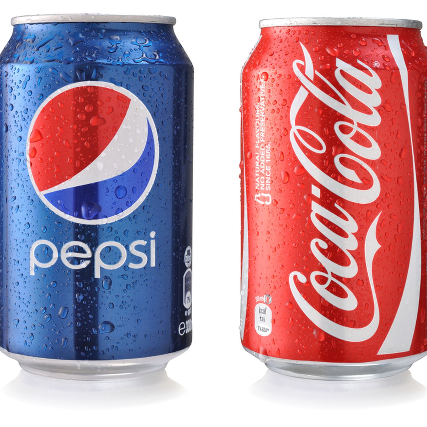

]

---

# Bertrand Competition: Example

]

---

# Bertrand Competition: Example

.pull-left[
- Demand for soda from .hi-red[Coke]:
 - `$Q$` if .red[`\$p_c\$`] `$<$` .blue[`\$p_p\$`]
]

---

# Bertrand Competition: Example

.pull-left[
- Demand for soda from .hi-red[Coke]:
 - `$Q$` if .red[`\$p_c\$`] `$<$` .blue[`\$p_p\$`]
 - `$\frac{Q}{2}$` if .red[`\$p_c\$`] `$=$` .blue[`\$p_p\$`]
]

---

# Bertrand Competition: Example

.pull-left[
- Demand for soda from .hi-red[Coke]:
 - `$Q$` if .red[`\$p_c\$`] `$<$` .blue[`\$p_p\$`]
 - `$\frac{Q}{2}$` if .red[`\$p_c\$`] `$=$` .blue[`\$p_p\$`]
 - `$0$` if .red[`\$p_c\$`] `$>$` .blue[`\$p_p\$`]
]

.pull-right[
<img src="2.3-slides_files/figure-html/unnamed-chunk-1-1.png" width="504" style="display: block; margin: auto;" />
]

---

# Bertrand Competition: Example

.pull-left[
- Demand for soda from .hi-blue[Pepsi]:
 - `$0$` if .red[`\$p_c\$`] `$<$` .blue[`\$p_p\$`]
 - `$\frac{Q}{2}$` if .red[`\$p_c\$`] `$=$` .blue[`\$p_p\$`]
 - `$Q$` if .red[`\$p_c\$`] `$>$` .blue[`\$p_p\$`]
]

---

# Bertrand Competition: Example

- The only way to sell *any* soda is to .hi-turquoise[match or beat your competitor's price]

]

---

# Bertrand Competition: Example

- The only way to sell *any* soda is to .hi-turquoise[match or beat your competitor's price]

- Suppose you are .hi-red[Coke]

- For a given .hi-blue[`\$p_p\$`], setting your price 
`$$\color{red}{p_c}=\color{blue}{p_p}-\epsilon$$`
for any arbitrary `$\epsilon > 0$` captures you the entire market `$Q$`

- Same for .hi-blue[Pepsi] for `$\color{blue}{p_c}$`

]

---

# Bertrand Competition: Example

- Won't charge `$p<MC$`, earn losses

- Firms continue undercutting one another until .hi-red[`\$p_c\$`] `$=$` .hi-blue[`\$p_p\$`] `$=MC$`
  - No incentive for either firm to raise or lower price, given other firm‘s price

- .hi-purple[Nash Equilibrium]: `$$\big( \color{red}{p_c = MC}, \color{blue}{p_p=MC} \big)$$`
  - Firms earn no profits!

]

---

# Bertrand Paradox

- .hi[Bertrand Paradox]: when firms compete on price, .hi-turquoise[the perfectly competitive outcome can be achieved with just 2 firms!]
  - `$p=MC$`
  - `$Q=Q_{(p=MC)}$`
  - `$\pi=0$`
  - `$L = \frac{p-MC}{p} = 0$`!

]

---

# Coke's Reaction Curve

.pull-left[
<img src="2.3-slides_files/figure-html/unnamed-chunk-2-1.png" width="504" style="display: block; margin: auto;" />
]

We can graph .hi-red[Coke]'s .hi-purple[reaction curve] to .hi-blue[Pepsi]'s price

]

---

# Coke's Reaction Curve

.pull-left[
<img src="2.3-slides_files/figure-html/unnamed-chunk-3-1.png" width="504" style="display: block; margin: auto;" />
]

We can graph .hi-red[Coke]'s .hi-purple[reaction curve] to .hi-blue[Pepsi]'s price

`$$\color{red}{p_c} = \begin{cases} \color{blue}{p_p} - \epsilon && \text{if } \color{blue}{p_p} > c\\ \color{blue}{p_p} && \text{if } \color{blue}{p_p} = c\\ \end{cases}$$`
- e.g. if .hi-blue[Pepsi] sets a price of .hi-blue[$1.00], .hi-red[Coke]'s best response is .hi-red[`\$$1.00-\epsilon\$`]

]

---

# Coke's Reaction Curve

.pull-left[
<img src="2.3-slides_files/figure-html/unnamed-chunk-4-1.png" width="504" style="display: block; margin: auto;" />
]

We can graph .hi-red[Coke]'s .hi-purple[reaction curve] to .hi-blue[Pepsi]'s price
`$$\color{red}{p_c} = \begin{cases} \color{blue}{p_p} - \epsilon && \text{if } \color{blue}{p_p} > c\\ \color{blue}{p_p} && \text{if } \color{blue}{p_p} = c\\ \end{cases}$$`

]

---

# Coke's Reaction Curve

.pull-left[
<img src="2.3-slides_files/figure-html/unnamed-chunk-5-1.png" width="504" style="display: block; margin: auto;" />
]

- e.g. if .hi-blue[Pepsi] sets a price of .hi-blue[$1.50], .hi-red[Coke]'s best response is .hi-red[`\$$1.50-\epsilon\$`]
- e.g. if .hi-blue[Pepsi] sets a price of .hi-blue[$1.50], .hi-red[Coke]'s best response is .hi-red[`\$$1.50-\epsilon\$`]
- e.g. if .hi-blue[Pepsi] sets a price of .hi-blue[$0.50], (MC) .hi-red[Coke]'s best response is .hi-red[`\$$0.50\$`] (MC)

]

---

# Pepsi's Reaction Curve

.pull-left[
<img src="2.3-slides_files/figure-html/unnamed-chunk-6-1.png" width="504" style="display: block; margin: auto;" />
]

We can graph .hi-blue[Pepsi]'s .hi-purple[reaction curve] to .hi-red[Coke]'s price

]
---

# Pepsi's Reaction Curve

.pull-left[
<img src="2.3-slides_files/figure-html/unnamed-chunk-7-1.png" width="504" style="display: block; margin: auto;" />
]

We can graph .hi-blue[Pepsi]'s .hi-purple[reaction curve] to .hi-red[Coke]'s price
`$$\color{blue}{p_p} = \begin{cases} \color{red}{p_c} - \epsilon && \text{if } \color{red}{p_c} > c\\ \color{red}{p_x} && \text{if } \color{red}{p_c} = c\\ \end{cases}$$`

- e.g. if .hi-red[Coke] sets a price of .hi-red[$1.00], .hi-blue[Pepsi]'s best response is .hi-blue[`\$$1.00-\epsilon\$`]

]

---

# Pepsi's Reaction Curve

.pull-left[
<img src="2.3-slides_files/figure-html/unnamed-chunk-8-1.png" width="504" style="display: block; margin: auto;" />
]

]

---

# Pepsi's Reaction Curve

.pull-left[
<img src="2.3-slides_files/figure-html/unnamed-chunk-9-1.png" width="504" style="display: block; margin: auto;" />
]

- e.g. if .hi-red[Coke] sets a price of .hi-red[$1.00], .hi-blue[Pepsi]'s best response is .hi-blue[`\$$1.00-\epsilon\$`]
- e.g. if .hi-red[Coke] sets a price of .hi-red[$1.50], .hi-blue[Pepsi]'s best response is .hi-blue[`\$$1.50-\epsilon\$`]
- e.g. if .hi-red[Coke] sets a price of .hi-red[$0.50] (MC),  .hi-blue[Pepsi]'s best response is .hi-blue[`\$$0.50\$`] (MC)

]

---

# Nash Equilibrium with Reaction Curves

.pull-left[
<img src="2.3-slides_files/figure-html/unnamed-chunk-10-1.png" width="504" style="display: block; margin: auto;" />
]

- Combine both curves on the same graph

- .hi-purple[Nash Equilibrium]: `$$\big( \color{red}{p_c = MC}, \color{blue}{p_p=MC} \big)$$`
    - Where both reaction curves intersect

- No longer an incentive to undercut or change price

]

---

# Bertrand Competition: The Market

- We can find the industry price & quantity of output (and profits), like in the Cournot model

- Here, set `$p=MC$`

`$$5-0.05Q = 0.50$$`

`$$Q^* = 90$$`

`$$q^\star_1 = q^\star_2 = 45$$`
--

$$P^* = c = \$0.50$$

`$$\pi_1 = \pi_2 = \Pi = 0$$`

---

# Bertrand Competition: The Market

---

# Cournot vs. Bertrand Competition

| Competition | `$q_i$` | `$Q$` | `$p$` | `$\pi_i$` |
|-------------|------:|----:|-----|--------:|
| Collusion   | 22.5  | 45.0  | $2.75 | $50.63 |
| Cournot     | 30.0  | 60.0  | $2.00 | $45.00 |
| Bertrand    | 45.0  | 90.0  | $0.50 | $0.00 |

- Output: `$Q_m < Q_c < Q_b$`
- Market price: `$P_b = c < P_c < P_m$`
- Profit: `$\pi_b = 0 < \pi_c < \pi_m$`

Where subscripts `$m$` is monopoly (collusion), `$c$` is Cournot, `$b$` is Bertrand

---

# Resolving the Bertrand Paradox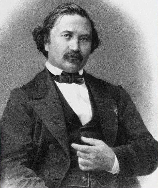

1822-1890
]
]
]

.right-column[
- The paradox happens due to pretty strict assumptions about the model
  - No capacity constraints 
  - Homogeneous goods; consumers *only* buy from the lower-priced seller

- We can extend the Bertrand model in a few ways and see the paradox resolved, we'll examine two:
  1. Bertrand competition with capacity constraints
  2. Bertrand competition with differentiated products

]

---

# Bertrand Competition with Capacity Constraints

---

# Capacity Constraints

- One way to resolve the paradox is to assume that each firm has .hi-purple[limited capacity] to produce, and cannot supply the entire market
  - certainly can't “flood” the market in a price war to drive price to `$MC$`

- Consider in the short run we assume capital is fixed

- Many goods/services are constrained by capacity: hotels, movie theaters, restaurants, etc.

]

---

# Capacity Constraints

`$$\begin{align*}q_1 &\leq k_1 \\
q_2 &\leq k_2 \\
k_1 + k_2 &< Q_D(c)\\
\end{align*}$$`

- Neither firm, nor both of them combined, can supply the entire market at marginal cost

- Cost per unit for firm `$i$` is `$c$` up for `$q_i <k_i$`, then increases rapidly (if not `$\infty)$`
]

.pull-right[
<img src="2.3-slides_files/figure-html/unnamed-chunk-12-1.png" width="504" style="display: block; margin: auto;" />

]

---

# Capacity Constraints Change the Game
 
.pull-left[

- Suppose .blue[Pepsi] charges a price `$\color{blue}{p_p} > c$`.

- .red[Coke] would simply have to charge `$\color{red}{p_c} = \color{blue}{p_p} - \epsilon$` to capture the market
  - But .red[Coke] does not have the capacity to serve the whole market!
  - Some customers would still buy .blue[Pepsi]!
  - So .blue[Pepsi] can charge a price above marginal cost

- `$\color{red}{p_c} = \color{blue}{p_p} = c$` is **not** a Nash equilibrium any more

]

---

# Capacity Constraints

.pull-left[
- Suppose .red[Coke] charges a price lower than .blue[Pepsi] `$\color{red}{p_c} < \color{blue}{p_p}$`.
 - But .red[Coke] does not have the capacity to serve the whole market, `$\color{red}{k_c} < Q_D(\color{red}{p_c})$`!
 - Some customers will still buy .blue[Pepsi]!

- Since neither firm can serve the whole market, we assume that they .hi[ration efficiently], that is, .red[Coke] only serve the customers with highest willingness to pay (first)

- .blue[Pepsi]'s residual demand is thus subtracting `$\color{red}{k_c}$` from the market demand
  - Note: the same as Cournot model residual demand, assuming `$q_c = q_k$`, i.e. Coke sells at capacity

]

.pull-right[
<img src="2.3-slides_files/figure-html/unnamed-chunk-13-1.png" width="504" style="display: block; margin: auto;" />

]

---

# Capacity Constraints

- If it charges `$\color{red}{p_c}<\color{blue}{p_p}$`, then it will sell `$\min \left\{Q_D(\color{red}{p_c}), \color{red}{k_c} \right\}$`
 - Either fulfills entire market demand (if its capacity `$\color{red}{k_c}$` exceeds demand); or its capacity (if `$\color{red}{k_c}$` is less than demand)
 - `$Q_D$` is quantity demanded at that price

- If it charges `$\color{red}{p_c}>\color{blue}{p_p}$`, then it will sell `$\min \left\{\color{red}{k_c}, Q_D(\color{red}{p_c})-\color{blue}{k_p} \right\}$`
  - .blue[Pepsi] sells its full capacity; .red[Coke] meets whatever demand is left (either sells its full capacity) or the remaining demand (if less than its capacity)

- If `$\color{red}{p_c}=\color{blue}{p_p}$` then we assume demand is allocated according to relative capacities, .red[Coke] sells `$\min \left\{\color{red}{k_c}, \frac{\color{red}{k_c}}{(\color{red}{k_c}+\color{blue}{k_c})D(p)}\right\}$`
  - e.g. if .red[Coke] has 45% of total industry capacity, it takes 45% of industry demand

]

---

# Nash Equilibrium Under Capacity Constraints

- .hi-purple[Case 1 (small capacities)]: Suppose each firm’s capacity is no larger than its Cournot best response to its competitor producing at capacity
`$$\begin{align*}k_c &\leq 30-0.5k_p \\
k_p &\leq 30-0.5k_c \\ \end{align*}$$`

]

.pull-right[
<img src="2.3-slides_files/figure-html/unnamed-chunk-14-1.png" width="504" style="display: block; margin: auto;" />
]

---

# Nash Equilibrium Under Capacity Constraints

.pull-left[
.smallest[
- .hi-purple[Nash equilibrium]: `$$p_c = p_ p = P(k_1+k_2)$$`
  - Each firm charges the same price, produces at capacity, and the price is the market demand at their combined capacities

- No incentive to lower price, can't produce more output (each at capacity)!
  
- No incentive to raise price either
  - Best response to other firm producing at `$k$` is your **Cournot best response**; but not possible (beyond your capacity); raising price makes you worse off (in fact you'd like to sell more and lower your price, but you can't!)

]
]

.pull-right[
<img src="2.3-slides_files/figure-html/unnamed-chunk-15-1.png" width="504" style="display: block; margin: auto;" />

]

---

# Nash Equilibrium Where Not Capacity Constrained

- .hi-orange[Case 2 (no capacity constraints)]: Suppose *each* firm’s capacity is sufficient to meet the entire market demand at marginal cost pricing

- **Nash equilibrium**: `$p_c = p_p = c$`

- Both firms flood the market, charging marginal cost (back to classic Bertrand game)
]

.pull-right[
<img src="2.3-slides_files/figure-html/unnamed-chunk-16-1.png" width="504" style="display: block; margin: auto;" />
]

---

# Bertrand Competition with Product Differentiation

---

# Product Differentiation

.pull-left[
.smaller[
- Now consider instead of homogenous goods, each seller is selling differentiated products (i.e. imperfect substitutes)
  - Consumers have preferences between Coke and Pepsi

- Same assumptions of Bertrand model:
  - Firms set their own prices simultaneously

- But now each firm faces its own downward-sloping demand curve
]
]
.pull-right[
.center[
![](../images/cokepepsi.jpg)
]
]

---

# Product Differentiation

- Suppose the demand for Coke and for Pepsi, respectively, are:
`$$q_c = 1.00-0.25p_c+0.25p_p \\
q_p = 1.00+0.25p_c-0.25p_p$$`

- Notice the positive relationship between `$p_p$` and `$q_c$` (and `$p_c$` and `$q_p$`): imperfect substitutes

]

---

# Product Differentiation

- Suppose the demand for Coke and for Pepsi, respectively, are:
`$$q_c = 1.00-0.25p_c+0.25p_p \\
q_p = 1.00+0.25p_c-0.25p_p$$`

- Notice the positive relationship between `$p_p$` and `$q_c$` (and `$p_c$` and `$q_p$`): imperfect substitutes

- Solving for Coke:

`$$MR_c = 1.00+0.25p_p-0.50p_c$$`

]

---

# Product Differentiation

- Solving for Coke:

`$$\begin{align*}
MR_c &= MC_c \\
1.00+0.25p_p-0.50p_c & = 0.50 \\ 
p_c & = 1.00 + 0.5p_p\end{align*}$$`

- Coke's reaction function to Pepsi's price
]

---

# Product Differentiation

- Solving for Coke:

`$$\begin{align*}
MR_c &= MC_c \\
1.00+0.25p_p-0.50p_c & = 0.50 \\ 
p_c & = 1.00 + 0.5p_p\end{align*}$$`

- Coke's reaction function to Pepsi's price

- Eqivalently for Pepsi:

`$$p_p = 1.00 + 0.5 p_c$$`
]

---

# Reaction Functions and Nash Equilibrium

---

# Reaction Functions and Nash Equilibrium: Algebraically

- .hi-purple[Nash Equilibrium] algebraically: plug one firm's reaction function into the other's

`$$\begin{align*}
p_{c}^*&=1.00+0.5p_{p}\\
p_{p}^*&=1.00+0.5p_{c}\\
\end{align*}$$`

`$$p_p^* = p_c^* = 2.00$$`

---

# Conjectural Variations

---

# Cournot vs Bertrand

![:scale 50%](../images/bertrand.jpg)
]
]
  
.right-column[

- Outcomes are *very* different between Cournot and Bertrand competition (with homogeneous products and no capacity constraints)
  - Market power & profits with Cournot; decreases with competitors and `$\varepsilon$`
  - Perfect competition with Bertrand

- Why? In Bertrand, firm anticipates that if it undercuts rival, can drive its sales to zero; but in Cournot it believes its rival will not change its output
]

---

# Cournot vs Bertrand

![:scale 50%](../images/bertrand.jpg)
]
]
  
.right-column[

.smallest[
- One interpretation: consider a two-stage game between firms with homogeneous products:
  1. Firms invest in capacity (setting `$k_i$`)
  2. Firms compete over price

- We can consider this once we learn more game theory

- Nash equilibrium: each firm invests in capacity `$k_i = q_i^c$`, equal to it's Cournot quantity; then prices equal to producing capacity
  - Limit capacity to reduce price competition in second stage! (Larger capacity `$\implies$` more aggressive price cutting)
  - In this case, Cournot model is a “shorthand” or reduced form of this 2 stage game
]
]

---

# Conjectural Variations

- Cournot's best response function is traditionally called a reaction function - from his discussion about how firms respond to another's output, *assuming the other firm does not change its output*

- Bowley (1924) calls this a .hi-purple[conjecture]: firm's belief about how its rivals will react to changes in its output

- Consider Cournot competition with homogenous goods, identical costs. Firm 1's marginal revenue is:

`$$MR_1 = P + \frac{\Delta P}{\Delta Q} \frac{\Delta Q}{\Delta q_1}q_1$$`

---

# Conjectural Variations

`$$MR_1(Q) = P + \frac{\Delta P}{\Delta Q} \color{#e64173}{\frac{\Delta Q}{\Delta q_1}}q_1$$`
- `$\color{#e64173}{\frac{\Delta Q}{\Delta q_1}}$` is the rate of change in *industry* output that firm 1 expects when it increases its output
  - `$\Delta Q = \Delta q_1 + \color{#6A5ACD}{\frac{\Delta q_2}{\Delta q_1}} \Delta q_1$`
  - where `$\color{#6A5ACD}{\frac{\Delta q_2}{\Delta q_1}}$` is Firm 1’s .hi-purple[conjecture] about **how Firm 2 will respond to Firm 1's output change**

- Divide everything by `$\Delta q_1$`:

`$$\frac{\Delta Q}{\Delta q_1} = 1 + \color{#6A5ACD}{\nu_1}$$`

- where `$\color{#6A5ACD}{\nu_1 = \frac{\Delta q_2}{\Delta q_1}}$`, Firm 1's conjecture

---

# Conjectural Variations

- Substituting this back in, we get

`$$MR_1(Q) = P(Q) + \frac{\Delta P(Q)}{\Delta Q} (1+ \color{#6A5ACD}{\nu_1})q_1$$`
- Equilibrium: each firm is profit-maximizing, given .hi-purple[its conjecture about its rival]

`$$P + \frac{\Delta P}{\Delta Q} (1+ \color{#6A5ACD}{\nu_1})q_1 = MC(q_1)$$`

And likewise for firm 2

`$$P + \frac{\Delta P}{\Delta Q} (1+ \color{#6A5ACD}{\nu_2})q_2 = MC(q_2)$$`

---

# Conjectural Variations

`$$P + \frac{\Delta P}{\Delta Q} (1+ \color{#6A5ACD}{\nu_1})q_1 = MC(q_1)$$`

- We can characterize effects of different conjectures on equilibrium output

- Larger values of `$\color{#6A5ACD}{\nu}$` (more aggressive response by other firm) reduce firm's `$MR(q)$` and therefore its output

---

# Conjectural Variations

- Assume a common conjecture between firms `$\color{#6A5ACD}{\nu}=\nu_1=\nu_2$`

]

.smaller[
- `$\nu = 0$`: the .hi-purple[Cournot conjecture].magenta[†] (reduces to the simple Cournot model)
 - rival does not change their output when you increase yours
]

.footnote[.magenta[†] Recall the definition of `\$MR(q)= p + \frac{\Delta p}{\Delta q}q\$`; or double the slope as demand.]

.smaller[
- `$\nu = -1$`: the .hi-purple[Bertrand conjecture]; firm is a price-taker, setting `$p=MC$`
  - rival reduces their output to offset each increase in yours (leaving price unchanged)

]

---

# Conjectural Variations

- Assume a common conjecture between firms `$\color{#6A5ACD}{\nu}=\nu_1=\nu_2$`

- `$\nu = 1$`: the .hi-purple[Collusive/monopoly conjecture], firm(s) acts like a monopolist over the industry (since `$2q_1$` is the total industry output)
  - rival changes their output exactly same as yours (collusive)
  - you can affect total industry output but not your market share (it will always remain constant)
  - one firm can't increase its profits at the expense of the other (i.e. cheating cartel is counterproductive)

`$$P + \frac{\Delta P}{\Delta Q} 2q_1 = MC(q_1)$$`

]

---

# Conjectural Variations: Flaws & Benefits

.pull-left[
.smallest[
- Logical flaw in the conjectural variations model: **assumes firms make decisions simultaneously**, not “reacting” to each other in real time!
  - We’ll deal with dynamic responses later

- But a useful empirical framework to explore market power and competitiveness
  - interpret and estimate `$\nu$` as a conduct parameter to see if industry performing closer to Cournot/Bertrand/Collusion
  - in general, the greater `$\nu$` is, the greater market power and markups are
]
]