1.5 — Monopoly I — Class Content
Overview
We begin looking at monopoly by discussing how a monopolist (as compared to a price-taking firm) chooses both its output and its price to maximize profits.
Readings
Recommended Readings
This is a part of our review of major production concepts from Microeconomics. You can consider looking at the following in the textbook if you are rusty or want to know more about these concepts:
- Ch. 2.1-2.2, 3.1 in Church & Ware, 2000
Practice
Today you will be working on practice problems:
Slides
Below, you can find the slides in two formats. Clicking the image will bring you to the html version of the slides in a new tab. The lower button will allow you to download a PDF version of the slides.
You can type h to see a special list of viewing options, and type o for an outline view of all the slides.
I suggest printing the slides beforehand and using them to take additional notes in class (not everything is in the slides)!
Appendix
Price Elasticity of Demand Refresher
Price elasticity of demand measures how much (in %) quantity demanded changes in response to a (1%) change in price.
\[\begin{align*} \epsilon_{q,p} &= \frac{\% \Delta q}{\% \Delta p}\\ &= \cfrac{\left(\frac{\Delta q}{q}\right)}{\left(\frac{\Delta p}{p}\right)}\\ &= \frac{\Delta q}{\Delta p} \times \frac{p}{q}\\ &= \frac{1}{slope} \times \frac{p}{q}\\ \end{align*}\]
| “Elastic” | “Unit Elastic” | “Inelastic” | |
|---|---|---|---|
| Intuitively: | Large response | Proportionate response | Little response |
| Mathematically: | \(\vert \epsilon_{q_D,p}\vert > 1\) | \(\vert \epsilon_{q_D,p}\vert = 1\) | \(\vert \epsilon_{q_D,p} \vert < 1\) |
| Numerator \(>\) Denominator | Numerator \(=\) Denominator | Numerator \(<\) Denominator | |
| A 1% change in \(p\) | More than 1% change in \(q_D\) | 1% change in \(q_D\) | Less than 1% change in \(q_D\) |
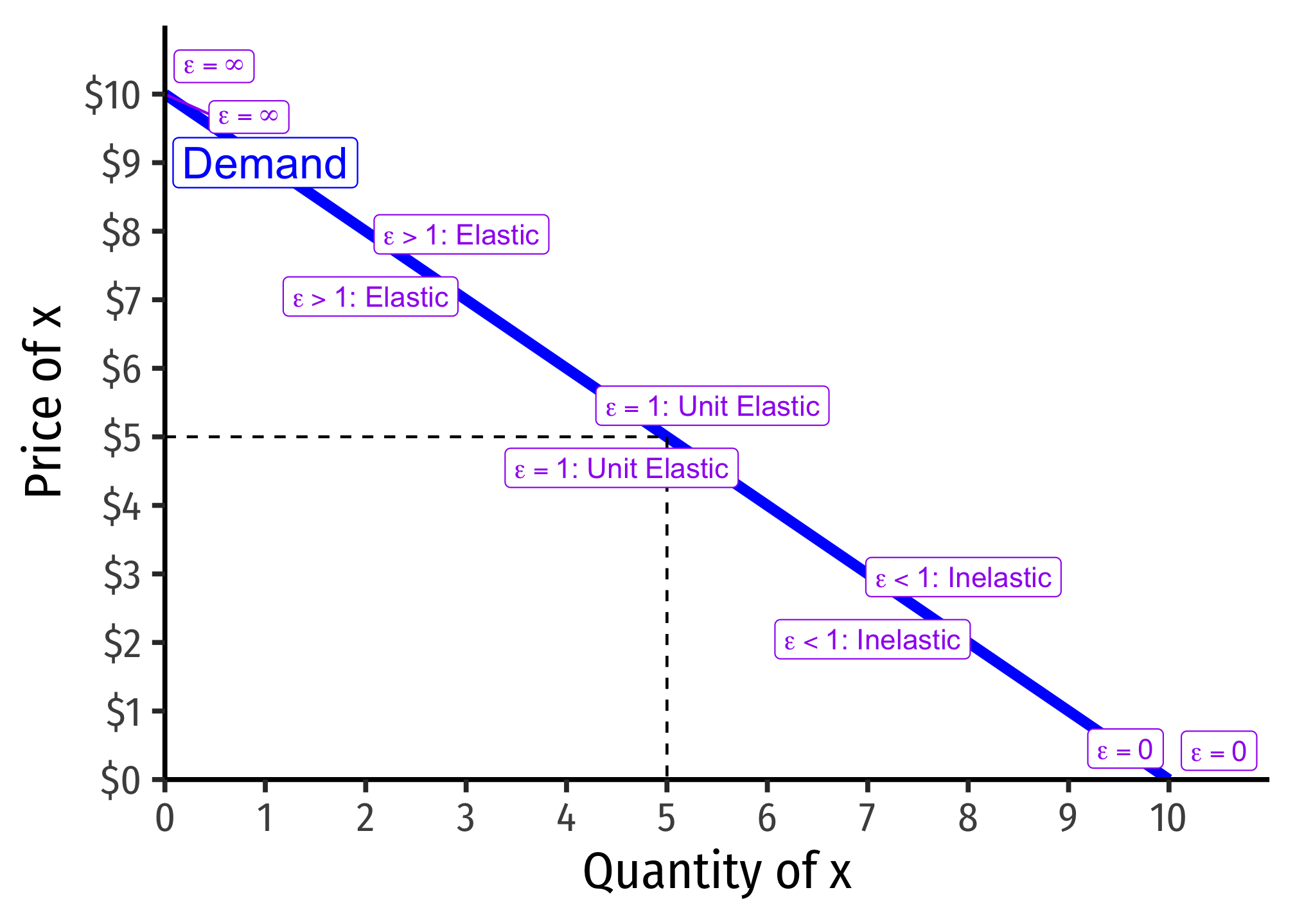
Price elasticity of demand changes along the demand curve:
Determinants of Price Elasticity
What determines how responsive your buying behavior is to a price change?
- More (fewer) substitutes \(\implies\) more (less) elastic
- Larger categories of products (less elastic) vs. specific brand (more elastic)
- Necessities (less elastic) vs. luxuries (more elastic)
- Large (more elastic) vs. small (less elastic) portion of budget
- More (less) time to adjust \(\implies\) more (less) elastic
Derivation of the Lerner Index
Marginal revenue is strongly related to the price elasticity of demand, which is \(E_{D}=\frac{\Delta q}{\Delta p} \times \frac{p}{q}\)1
We derived marginal revenue (in the slides) as: \[MR(q)=p+\frac{\Delta p}{\Delta q}q\]
Firms will always maximize profits where:
\[\begin{align*} MR(q)&=MC(q) && \text{Profit-max output}\\ p+\bigg(\frac{\Delta p}{\Delta q}\bigg)q&=MC(q) && \text{Definition of } MR(q)\\ p+\bigg(\frac{\Delta p}{\Delta q}\bigg) q \times \frac{p}{p}&=\frac{MR(q)}{p} && \text{Multiplying the left by } \frac{p}{p} \text{ (i.e. 1)}\\ p+\underbrace{\bigg(\frac{\Delta p}{\Delta q}\times \frac{q}{p} \bigg)}_{\frac{1}{\epsilon}} \times p &=MC(q) && \text{Rearranging the left}\\ p+\frac{1}{\epsilon} \times p &=MC(q) && \text{Recognize price elasticity } \epsilon=\frac{\Delta q}{\Delta p} \times \frac{p}{q}\\ p &=MC(q) - \frac{1}{\epsilon} p && \text{Subtract }\frac{1}{\epsilon}p \text{ from both sides}\\ p-MC(q) &= -\frac{1}{\epsilon} p && \text{Subtract }MC(q) \text{ from both sides}\\ \frac{p-MC(q)}{p} &= -\frac{1}{\epsilon} && \text{Divide both sides by }p\\ \end{align*}\]
The left side gives us the fraction of price that is markup \(\left(\frac{p-MC(q)}{p}\right)\), and the right side shows this is inversely related to price elasticity of demand.
Footnotes
I sometimes simplify it as \(E_{D}=\frac{1}{slope} \times \frac{p}{q}\), where “slope” is the slope of the inverse demand curve (graph), since the slope is \(\frac{\Delta p}{\Delta q} = \frac{rise}{run}\).↩︎
